

 **1. Descriptive Analysis**
Data Cleaning: Removing data that are incorrect, incomplete, missing, or duplicate values is called data cleaning. It increases the accuracy of data.
**1. Descriptive Analysis**
Data Cleaning: Removing data that are incorrect, incomplete, missing, or duplicate values is called data cleaning. It increases the accuracy of data.
 > Our raw dataset has 506 rows × 20 columns, after data cleaning, I have changed it to 506 rows × 14 columns

> CRIM, ZN, TAX have significantly different mean and median, signifying extreme values (3rd-4th Quartile), which is skewing the mean towards the right.
**2. Exploratory analysis**
> In this section, I check the correlations with our dependent variable CMEDV
> Our raw dataset has 506 rows × 20 columns, after data cleaning, I have changed it to 506 rows × 14 columns

> CRIM, ZN, TAX have significantly different mean and median, signifying extreme values (3rd-4th Quartile), which is skewing the mean towards the right.
**2. Exploratory analysis**
> In this section, I check the correlations with our dependent variable CMEDV
 > .00-.19 “very weak” | .20-.39 “weak” | .40-.59 “moderate” | .60-.79 “strong” | .80-1.0 “very strong”
> With CMEDV
Very Weak - CHAS, B
Weak - RAD
Moderate - CRIM, ZN, INDUS, NOX, AGE, DIS, TAX, PTRATIO
Strong - RM
Very Strong - LSTAT
It is interesting to note the highest correlations of dis with crime, indus, nox, and age. Also between indus and nox, as well as those between tax and rad and tax and indus. It makes sense that nitrogen oxide levels and tax levels are highest near industrial areas. These are possible sources of multicollinearity, each explaining the same thing as far as how they affect variation in CMEDV.
Related to CMEDV itself, it is found that the average number of rooms has the highest positive correlation, while the pupil-teacher ratio and lstat have the highest negative correlations.
> .00-.19 “very weak” | .20-.39 “weak” | .40-.59 “moderate” | .60-.79 “strong” | .80-1.0 “very strong”
> With CMEDV
Very Weak - CHAS, B
Weak - RAD
Moderate - CRIM, ZN, INDUS, NOX, AGE, DIS, TAX, PTRATIO
Strong - RM
Very Strong - LSTAT
It is interesting to note the highest correlations of dis with crime, indus, nox, and age. Also between indus and nox, as well as those between tax and rad and tax and indus. It makes sense that nitrogen oxide levels and tax levels are highest near industrial areas. These are possible sources of multicollinearity, each explaining the same thing as far as how they affect variation in CMEDV.
Related to CMEDV itself, it is found that the average number of rooms has the highest positive correlation, while the pupil-teacher ratio and lstat have the highest negative correlations.

 * CRIM, ZN, LSTAT, NOX is right-skewed
* PTRATIO, B is left-skewed
* The right-skewed distribution suggests that a log transformation would be appropriate. The left-skewed distribution of ptratio suggests that squaring it could make for a better fit.
* To fit a regression model for the first time, the log transformation will only be applied to CMEDV to determine whether it does indeed provide a better fit.
**3. Multivariate Linear Regression**
In this section, I fit the data to the ordinary least squares (OLS) model and compare the results before and after implementing the Log Transformation.
Here is the OLS Regression Results using Log Transformation of CMEDV:
* CRIM, ZN, LSTAT, NOX is right-skewed
* PTRATIO, B is left-skewed
* The right-skewed distribution suggests that a log transformation would be appropriate. The left-skewed distribution of ptratio suggests that squaring it could make for a better fit.
* To fit a regression model for the first time, the log transformation will only be applied to CMEDV to determine whether it does indeed provide a better fit.
**3. Multivariate Linear Regression**
In this section, I fit the data to the ordinary least squares (OLS) model and compare the results before and after implementing the Log Transformation.
Here is the OLS Regression Results using Log Transformation of CMEDV:
 Here is the OLS Regression Results without using Log Transformation of CMEDV:
 Thus, the log transformation of CMEDV is indeed appropriate. Now, the predictors that are not statistically significant can be removed from the model. They are INDUS, AGE, and ZN. Moreover, for the purpose of this report, the variables TAX and RAD are not of interest, since they are highly correlated with proximity to industries which itself is not significant.
Then, I calculated variance inflation factors for all variables. As all values are less than 5 except TAX & RAD, there are no issues of multicollinearity.
Thus, the log transformation of CMEDV is indeed appropriate. Now, the predictors that are not statistically significant can be removed from the model. They are INDUS, AGE, and ZN. Moreover, for the purpose of this report, the variables TAX and RAD are not of interest, since they are highly correlated with proximity to industries which itself is not significant.
Then, I calculated variance inflation factors for all variables. As all values are less than 5 except TAX & RAD, there are no issues of multicollinearity.
 **4. Feature Selection**
* So far, I am using 14 features, including CMEDV, CRIM, ZN, INDUS, CHAS, NOX, RM, AGE, DIS, RAD, TAX, PTRATIO, B, and LSTAT.
* Based on the previous section, I removed 5 variables: ZN, INDUS, AGE, RAD, and TAX.
* Thus, our final selected features are CMEDV, CRIM, CHAS, NOX, RM, DIS, PTRATIO, B, LSTAT.
**5. Checking Normality for Selected Variables**
I check Normality for all selected features by creating a Q-Q plot for each one of them.
**4. Feature Selection**
* So far, I am using 14 features, including CMEDV, CRIM, ZN, INDUS, CHAS, NOX, RM, AGE, DIS, RAD, TAX, PTRATIO, B, and LSTAT.
* Based on the previous section, I removed 5 variables: ZN, INDUS, AGE, RAD, and TAX.
* Thus, our final selected features are CMEDV, CRIM, CHAS, NOX, RM, DIS, PTRATIO, B, LSTAT.
**5. Checking Normality for Selected Variables**
I check Normality for all selected features by creating a Q-Q plot for each one of them.
 * CRIM, NOX, DIS, LSTAT are right skewed, indicating that a log transformation would be appropriate.
* LSTAT, B, PTRATIO are left skewed, suggesting that a square transformation could make a better fit.
**6. Feature Transformation**
As stated in the previous section, I implement log transformation on variables: CRIM, NOX, DIS, and LSTAT, and do square transformation on LSTAT, B, and PTRATIO. Again, I check their Normality by creating a Q-Q plot for each one of them.
* CRIM, NOX, DIS, LSTAT are right skewed, indicating that a log transformation would be appropriate.
* LSTAT, B, PTRATIO are left skewed, suggesting that a square transformation could make a better fit.
**6. Feature Transformation**
As stated in the previous section, I implement log transformation on variables: CRIM, NOX, DIS, and LSTAT, and do square transformation on LSTAT, B, and PTRATIO. Again, I check their Normality by creating a Q-Q plot for each one of them.
 From this chart, I can see that there is a bit improvement in Normality of all the transformed variables.
**7. Removing Outliers and high influence points**
To further improve their Normality, I need to remove Outliers and High Influence Points.
From this chart, I can see that there is a bit improvement in Normality of all the transformed variables.
**7. Removing Outliers and high influence points**
To further improve their Normality, I need to remove Outliers and High Influence Points.
 Then, I create a plot of Leverage and Studentized Residuals.
 After that, I create a plot of large Leverage and large Studentized Residuals, using residual squared to restrict the graph but preserve the relative position of observations.

 **8. Linear Regression**
In this I find linear regression summary of r2 score and standard deviation using, cross validation techniques.
**8. Linear Regression**
In this I find linear regression summary of r2 score and standard deviation using, cross validation techniques.
 Find the value of r2 score, adjusted r2 score and root mean squared error value using testing and training datasets.
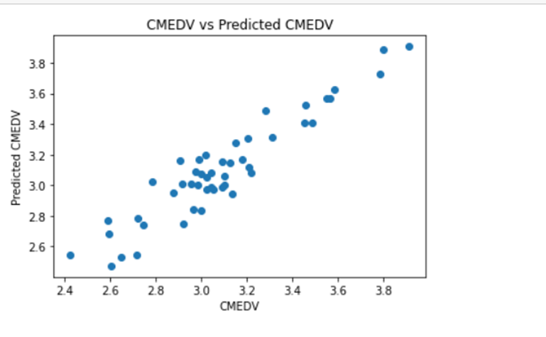
 Create scatter plot for actual CMEDV and predicted CMEDV to see the difference between them.
 Checking Residuals:
 **9. Support Vector Machine**
In this I find summary of r2 score and standard deviation using, Support Vector Machine Regressor.
**9. Support Vector Machine**
In this I find summary of r2 score and standard deviation using, Support Vector Machine Regressor.
 Find the value of r2 score, adjusted r2 score and root mean squared error value using testing and training datasets.
 Create scatter plot for actual CMEDV and predicted CMEDV to see the difference between them.
 Checking Residuals:
 **10. Random Forest**
In this I find summary of r2 score and standard deviation using, Random Forest Regressor.
**10. Random Forest**
In this I find summary of r2 score and standard deviation using, Random Forest Regressor.
 Evaluating the model to check the r2, adjusted r2 score and root means square error value with 2 datasets such as training and testing datasets.
 Visualizing the differences between actual prices and predicted values. Create scatter plot for actual CMEDV and predicted CMEDV to see the difference between them.
 Also, creating scatter plot to check predicted vs residual.
 **11. XGBOOST Regressor**
In this I find summary of r2 score and standard deviation using, XGBoost Regressor.
**11. XGBOOST Regressor**
In this I find summary of r2 score and standard deviation using, XGBoost Regressor.
 Evaluating the model to check the r2, adjusted r2 score and root means square error value with 2 datasets such as training and testing datasets.
 Visualizing the differences between actual prices and predicted values. Create scatter plot for actual CMEDV and predicted CMEDV to see the difference between them.
 Also, creating scatter plot to check predicted vs residual.
 **12. Evaluation and Comparison of Models**
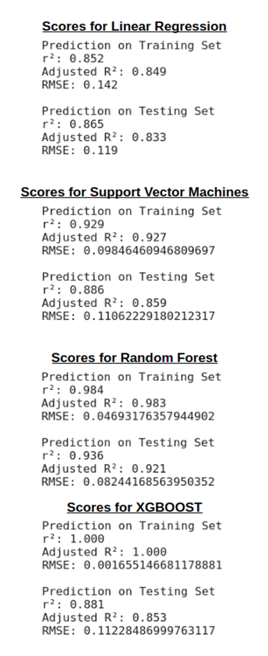 > Random Forest surpasses all the other models I’ve used.
It explains 92.1% of the variance in our dataset.
Hence, Random Forest is best for prediction as it’s accuracy is better than other models here.
**Ranking**:
1. Random Forest
2. XGBoost
3. Support Vector Machines
4. Linear Regression
### References
1. https://www.analyticsvidhya.com/blog/2020/03/support-vector-regression-tutorial-for-machine-learning/
2. https://www.analyticsvidhya.com/blog/2021/06/understanding-random-forest/
3. https://www.analyticssteps.com/blogs/introduction-xgboost-algorithm-classification-and-regression
> Random Forest surpasses all the other models I’ve used.
It explains 92.1% of the variance in our dataset.
Hence, Random Forest is best for prediction as it’s accuracy is better than other models here.
**Ranking**:
1. Random Forest
2. XGBoost
3. Support Vector Machines
4. Linear Regression
### References
1. https://www.analyticsvidhya.com/blog/2020/03/support-vector-regression-tutorial-for-machine-learning/
2. https://www.analyticsvidhya.com/blog/2021/06/understanding-random-forest/
3. https://www.analyticssteps.com/blogs/introduction-xgboost-algorithm-classification-and-regression