gtav-racebot-bc.ipynb
GTA V Racebot via Behavioural Cloning
This notebook trains a racebot for GTA V for a simple race track (https://www.gta5-mods.com/maps/formula-1-formula-e-circuit). We use behavioural cloning from imitation learning, in which the model learns a policy by mimicking the demonstrations (i.e., transforms the problem to a supervised learning problem). The states are defined as the speed of the car & raycast distances & the actions are discrete values for throttle & steering.
- EDA
- Train
- Conclusion
import pandas as pd
import numpy as np
import tensorflow as tf
from tensorflow import keras
from sklearn.model_selection import train_test_split
from sklearn.preprocessing import StandardScaler
import matplotlib.pyplot as plt
2025-11-15 17:16:45.345169: E external/local_xla/xla/stream_executor/cuda/cuda_fft.cc:477] Unable to register cuFFT factory: Attempting to register factory for plugin cuFFT when one has already been registered
WARNING: All log messages before absl::InitializeLog() is called are written to STDERR
E0000 00:00:1763227005.608597      48 cuda_dnn.cc:8310] Unable to register cuDNN factory: Attempting to register factory for plugin cuDNN when one has already been registered
E0000 00:00:1763227005.683645      48 cuda_blas.cc:1418] Unable to register cuBLAS factory: Attempting to register factory for plugin cuBLAS when one has already been registered


---------------------------------------------------------------------------

AttributeError                            Traceback (most recent call last)

AttributeError: 'MessageFactory' object has no attribute 'GetPrototype'


---------------------------------------------------------------------------

AttributeError                            Traceback (most recent call last)

AttributeError: 'MessageFactory' object has no attribute 'GetPrototype'


---------------------------------------------------------------------------

AttributeError                            Traceback (most recent call last)

AttributeError: 'MessageFactory' object has no attribute 'GetPrototype'


---------------------------------------------------------------------------

AttributeError                            Traceback (most recent call last)

AttributeError: 'MessageFactory' object has no attribute 'GetPrototype'


---------------------------------------------------------------------------

AttributeError                            Traceback (most recent call last)

AttributeError: 'MessageFactory' object has no attribute 'GetPrototype'
FILE_PATH = '/kaggle/input/racing-data-bc-1/racing_data_20251111_115450.csv'
1. EDA
We must look for imbalances in the labels, since the track has long straights, our data will have less turn data.
df = pd.read_csv(FILE_PATH, index_col=False)
print(f"Samples: {len(df)}")
print(df.head())
print(df.describe())
Samples: 84286
      speed    ray_0    ray_1    ray_2    ray_3    ray_4    ray_5    ray_6  \
0  0.006423  13.3434  17.9467  33.5831  79.1044  29.4587  15.6063  11.5635
1  0.006048  13.3434  17.9468  33.5835  79.1041  29.4584  15.6063  11.5635
2  0.006314  13.3434  17.9467  33.5832  79.1041  29.4584  15.6063  11.5635
3  0.006494  13.3434  17.9467  33.5832  79.1044  29.4587  15.6063  11.5635
4  0.006364  13.3434  17.9467  33.5832  79.1044  29.4587  15.6063  11.5635

   steering  throttle
0       0.0       0.0
1       0.0       0.0
2       0.0       0.0
3       0.0       0.0
4       0.0       0.0
              speed         ray_0         ray_1         ray_2         ray_3  \
count  84286.000000  84286.000000  84286.000000  84286.000000  84286.000000
mean      40.815017     13.415752     18.091388     42.415051     87.546020
std        5.639448      9.768494     10.486268     24.504446     32.479647
min        0.003145      2.576450      3.434760      6.310280     19.345600
25%       38.041825     10.125800     13.935925     27.932875     54.100275
50%       41.566050     12.135500     16.617450     33.378150     93.782500
75%       44.620075     14.150575     19.061475     44.901200    120.000000
max       51.009200    120.000000    120.000000    120.000000    120.000000

              ray_4         ray_5         ray_6      steering      throttle
count  84286.000000  84286.000000  84286.000000  84286.000000  84286.000000
mean      33.908074     16.857788     12.871764     -0.074980      0.855378
std       16.383217      4.444279      5.221268      0.405839      0.334569
min        8.011750      4.165840      3.043060     -1.000000      0.000000
25%       26.174450     14.105825     10.438725      0.000000      1.000000
50%       29.137350     16.105800     12.016250      0.000000      1.000000
75%       34.616525     19.263150     14.863150      0.000000      1.000000
max      120.000000     70.365300    120.000000      1.000000      1.000000
df = df[df['speed'] > 5.0] # get rid of crashes or stationary
print(f"Samples: {len(df)}")
Samples: 84133
print(f"Left turns (< -0.1): {(df['steering'] < -0.1).sum()}")
print(f"Straight (±0.1): {(df['steering'].abs() <= 0.1).sum()}")
print(f"Right turns (> 0.1): {(df['steering'] > 0.1).sum()}")
Left turns (< -0.1): 15491
Straight (±0.1): 59781
Right turns (> 0.1): 8861
straight = df[df['steering'].abs() < 0.1]
turning = df[df['steering'].abs() >= 0.1]

if len(straight) > len(turning) * 2:
    straight_sampled = straight.sample(n=len(turning) * 2, random_state=42)
    df = pd.concat([straight_sampled, turning])
    df = df.sample(frac=1, random_state=42).reset_index(drop=True)
    print(f"After balancing: {len(df)}")
After balancing: 73056
throttle_on = df[df['throttle'] > 0.1]
throttle_off = df[df['throttle'] <= 0.1]
if len(throttle_on) > len(throttle_off) * 2:
    throttle_on_sampled = throttle_on.sample(n=len(throttle_off) * 2, random_state=42)
    df = pd.concat([throttle_on_sampled, throttle_off])
    print(f"After balancing: {len(df)}")
After balancing: 27606
2. Training
We will create a simple MLP w/ just 2 layers.
X = df[['speed', 'ray_0', 'ray_1', 'ray_2', 'ray_3', 'ray_4', 'ray_5', 'ray_6']].values
y = df[['steering', 'throttle']].values
scaler_X = StandardScaler()
X_scaled = scaler_X.fit_transform(X)

print(scaler_X.mean_)
print(scaler_X.scale_)
[40.31387887 13.3171938  17.94204432 44.73560258 77.80768833 35.56498163
 16.78186832 12.84412013]
[ 5.47637981  9.25261478  9.72122038 24.71908633 32.80978699 18.13965501
  4.19510602  5.41073173]
import joblib
joblib.dump(scaler_X, 'scaler.pkl')

print(scaler_X.mean_)
print(scaler_X.scale_)
[40.31387887 13.3171938  17.94204432 44.73560258 77.80768833 35.56498163
 16.78186832 12.84412013]
[ 5.47637981  9.25261478  9.72122038 24.71908633 32.80978699 18.13965501
  4.19510602  5.41073173]
X_train, X_test, y_train, y_test = train_test_split(
    X_scaled, y, test_size=0.2, random_state=42
)
model = keras.Sequential([
    keras.layers.Input(shape=(8,)),  # speed + 7 rays
    keras.layers.Dense(64, activation='relu'),
    keras.layers.Dropout(0.3),

    keras.layers.Dense(64, activation='relu'),
    keras.layers.Dropout(0.2),

    # tanh for steering (-1 to 1), sigmoid for throttle (0 to 1)
    keras.layers.Dense(2, activation='linear')  # we'll split outputs
])
model.compile(
    optimizer=keras.optimizers.Adam(learning_rate=0.001),
    loss='mse',
    metrics=['mae']
)

model.summary()
Model: "sequential_2"
┏━━━━━━━━━━━━━━━━━━━━━━━━━━━━━━━━━┳━━━━━━━━━━━━━━━━━━━━━━━━┳━━━━━━━━━━━━━━━┓
┃ Layer (type)                    ┃ Output Shape           ┃       Param # ┃
┡━━━━━━━━━━━━━━━━━━━━━━━━━━━━━━━━━╇━━━━━━━━━━━━━━━━━━━━━━━━╇━━━━━━━━━━━━━━━┩
│ dense_6 (Dense)                 │ (None, 64)             │           576 │
├─────────────────────────────────┼────────────────────────┼───────────────┤
│ dropout_4 (Dropout)             │ (None, 64)             │             0 │
├─────────────────────────────────┼────────────────────────┼───────────────┤
│ dense_7 (Dense)                 │ (None, 64)             │         4,160 │
├─────────────────────────────────┼────────────────────────┼───────────────┤
│ dropout_5 (Dropout)             │ (None, 64)             │             0 │
├─────────────────────────────────┼────────────────────────┼───────────────┤
│ dense_8 (Dense)                 │ (None, 32)             │         2,080 │
├─────────────────────────────────┼────────────────────────┼───────────────┤
│ dropout_6 (Dropout)             │ (None, 32)             │             0 │
├─────────────────────────────────┼────────────────────────┼───────────────┤
│ dense_9 (Dense)                 │ (None, 2)              │            66 │
└─────────────────────────────────┴────────────────────────┴───────────────┘
Total params: 6,882 (26.88 KB)
Trainable params: 6,882 (26.88 KB)
Non-trainable params: 0 (0.00 B)
early_stop = keras.callbacks.EarlyStopping(
    monitor='val_loss',
    patience=5,
    restore_best_weights=True
)

history = model.fit(
    X_train, y_train,
    validation_data=(X_test, y_test),
    epochs=50,
    batch_size=64,
    callbacks=[early_stop],
    verbose=1
)
Epoch 1/50
[1m346/346[0m [32m━━━━━━━━━━━━━━━━━━━━[0m[37m[0m [1m3s[0m 3ms/step - loss: 0.2429 - mae: 0.3737 - val_loss: 0.1314 - val_mae: 0.2881
Epoch 2/50
[1m346/346[0m [32m━━━━━━━━━━━━━━━━━━━━[0m[37m[0m [1m1s[0m 3ms/step - loss: 0.1481 - mae: 0.3034 - val_loss: 0.1221 - val_mae: 0.2713
Epoch 3/50
[1m346/346[0m [32m━━━━━━━━━━━━━━━━━━━━[0m[37m[0m [1m1s[0m 3ms/step - loss: 0.1324 - mae: 0.2827 - val_loss: 0.1157 - val_mae: 0.2683
Epoch 4/50
[1m346/346[0m [32m━━━━━━━━━━━━━━━━━━━━[0m[37m[0m [1m1s[0m 3ms/step - loss: 0.1265 - mae: 0.2729 - val_loss: 0.1093 - val_mae: 0.2550
Epoch 5/50
[1m346/346[0m [32m━━━━━━━━━━━━━━━━━━━━[0m[37m[0m [1m1s[0m 3ms/step - loss: 0.1186 - mae: 0.2585 - val_loss: 0.1049 - val_mae: 0.2390
Epoch 6/50
[1m346/346[0m [32m━━━━━━━━━━━━━━━━━━━━[0m[37m[0m [1m1s[0m 3ms/step - loss: 0.1158 - mae: 0.2523 - val_loss: 0.1029 - val_mae: 0.2391
Epoch 7/50
[1m346/346[0m [32m━━━━━━━━━━━━━━━━━━━━[0m[37m[0m [1m1s[0m 3ms/step - loss: 0.1135 - mae: 0.2489 - val_loss: 0.1007 - val_mae: 0.2273
Epoch 8/50
[1m346/346[0m [32m━━━━━━━━━━━━━━━━━━━━[0m[37m[0m [1m1s[0m 3ms/step - loss: 0.1105 - mae: 0.2426 - val_loss: 0.0989 - val_mae: 0.2279
Epoch 9/50
[1m346/346[0m [32m━━━━━━━━━━━━━━━━━━━━[0m[37m[0m [1m1s[0m 3ms/step - loss: 0.1085 - mae: 0.2389 - val_loss: 0.0972 - val_mae: 0.2190
Epoch 10/50
[1m346/346[0m [32m━━━━━━━━━━━━━━━━━━━━[0m[37m[0m [1m1s[0m 3ms/step - loss: 0.1065 - mae: 0.2367 - val_loss: 0.0977 - val_mae: 0.2284
Epoch 11/50
[1m346/346[0m [32m━━━━━━━━━━━━━━━━━━━━[0m[37m[0m [1m1s[0m 3ms/step - loss: 0.1047 - mae: 0.2334 - val_loss: 0.0952 - val_mae: 0.2186
Epoch 12/50
[1m346/346[0m [32m━━━━━━━━━━━━━━━━━━━━[0m[37m[0m [1m1s[0m 3ms/step - loss: 0.1069 - mae: 0.2360 - val_loss: 0.0948 - val_mae: 0.2224
Epoch 13/50
[1m346/346[0m [32m━━━━━━━━━━━━━━━━━━━━[0m[37m[0m [1m1s[0m 3ms/step - loss: 0.1029 - mae: 0.2297 - val_loss: 0.0936 - val_mae: 0.2166
Epoch 14/50
[1m346/346[0m [32m━━━━━━━━━━━━━━━━━━━━[0m[37m[0m [1m1s[0m 3ms/step - loss: 0.1013 - mae: 0.2267 - val_loss: 0.0930 - val_mae: 0.2118
Epoch 15/50
[1m346/346[0m [32m━━━━━━━━━━━━━━━━━━━━[0m[37m[0m [1m1s[0m 3ms/step - loss: 0.1023 - mae: 0.2282 - val_loss: 0.0930 - val_mae: 0.2073
Epoch 16/50
[1m346/346[0m [32m━━━━━━━━━━━━━━━━━━━━[0m[37m[0m [1m1s[0m 3ms/step - loss: 0.1021 - mae: 0.2272 - val_loss: 0.0917 - val_mae: 0.2050
Epoch 17/50
[1m346/346[0m [32m━━━━━━━━━━━━━━━━━━━━[0m[37m[0m [1m1s[0m 3ms/step - loss: 0.1000 - mae: 0.2232 - val_loss: 0.0906 - val_mae: 0.2046
Epoch 18/50
[1m346/346[0m [32m━━━━━━━━━━━━━━━━━━━━[0m[37m[0m [1m1s[0m 3ms/step - loss: 0.0994 - mae: 0.2233 - val_loss: 0.0906 - val_mae: 0.2009
Epoch 19/50
[1m346/346[0m [32m━━━━━━━━━━━━━━━━━━━━[0m[37m[0m [1m1s[0m 3ms/step - loss: 0.0998 - mae: 0.2223 - val_loss: 0.0901 - val_mae: 0.2041
Epoch 20/50
[1m346/346[0m [32m━━━━━━━━━━━━━━━━━━━━[0m[37m[0m [1m1s[0m 3ms/step - loss: 0.0992 - mae: 0.2223 - val_loss: 0.0904 - val_mae: 0.2074
Epoch 21/50
[1m346/346[0m [32m━━━━━━━━━━━━━━━━━━━━[0m[37m[0m [1m1s[0m 3ms/step - loss: 0.0960 - mae: 0.2177 - val_loss: 0.0898 - val_mae: 0.2002
Epoch 22/50
[1m346/346[0m [32m━━━━━━━━━━━━━━━━━━━━[0m[37m[0m [1m1s[0m 3ms/step - loss: 0.0968 - mae: 0.2183 - val_loss: 0.0901 - val_mae: 0.2064
Epoch 23/50
[1m346/346[0m [32m━━━━━━━━━━━━━━━━━━━━[0m[37m[0m [1m1s[0m 3ms/step - loss: 0.0980 - mae: 0.2209 - val_loss: 0.0891 - val_mae: 0.2014
Epoch 24/50
[1m346/346[0m [32m━━━━━━━━━━━━━━━━━━━━[0m[37m[0m [1m1s[0m 3ms/step - loss: 0.0967 - mae: 0.2191 - val_loss: 0.0894 - val_mae: 0.2065
Epoch 25/50
[1m346/346[0m [32m━━━━━━━━━━━━━━━━━━━━[0m[37m[0m [1m1s[0m 3ms/step - loss: 0.0980 - mae: 0.2199 - val_loss: 0.0882 - val_mae: 0.1997
Epoch 26/50
[1m346/346[0m [32m━━━━━━━━━━━━━━━━━━━━[0m[37m[0m [1m1s[0m 3ms/step - loss: 0.0972 - mae: 0.2193 - val_loss: 0.0877 - val_mae: 0.1980
Epoch 27/50
[1m346/346[0m [32m━━━━━━━━━━━━━━━━━━━━[0m[37m[0m [1m1s[0m 3ms/step - loss: 0.0961 - mae: 0.2181 - val_loss: 0.0885 - val_mae: 0.2036
Epoch 28/50
[1m346/346[0m [32m━━━━━━━━━━━━━━━━━━━━[0m[37m[0m [1m1s[0m 3ms/step - loss: 0.0959 - mae: 0.2183 - val_loss: 0.0873 - val_mae: 0.1999
Epoch 29/50
[1m346/346[0m [32m━━━━━━━━━━━━━━━━━━━━[0m[37m[0m [1m1s[0m 3ms/step - loss: 0.0965 - mae: 0.2185 - val_loss: 0.0873 - val_mae: 0.1959
Epoch 30/50
[1m346/346[0m [32m━━━━━━━━━━━━━━━━━━━━[0m[37m[0m [1m1s[0m 3ms/step - loss: 0.0941 - mae: 0.2147 - val_loss: 0.0875 - val_mae: 0.1998
Epoch 31/50
[1m346/346[0m [32m━━━━━━━━━━━━━━━━━━━━[0m[37m[0m [1m1s[0m 3ms/step - loss: 0.0961 - mae: 0.2172 - val_loss: 0.0864 - val_mae: 0.1936
Epoch 32/50
[1m346/346[0m [32m━━━━━━━━━━━━━━━━━━━━[0m[37m[0m [1m1s[0m 3ms/step - loss: 0.0938 - mae: 0.2133 - val_loss: 0.0869 - val_mae: 0.1994
Epoch 33/50
[1m346/346[0m [32m━━━━━━━━━━━━━━━━━━━━[0m[37m[0m [1m1s[0m 3ms/step - loss: 0.0934 - mae: 0.2137 - val_loss: 0.0860 - val_mae: 0.2001
Epoch 34/50
[1m346/346[0m [32m━━━━━━━━━━━━━━━━━━━━[0m[37m[0m [1m1s[0m 3ms/step - loss: 0.0933 - mae: 0.2137 - val_loss: 0.0862 - val_mae: 0.1978
Epoch 35/50
[1m346/346[0m [32m━━━━━━━━━━━━━━━━━━━━[0m[37m[0m [1m1s[0m 3ms/step - loss: 0.0934 - mae: 0.2136 - val_loss: 0.0870 - val_mae: 0.2000
Epoch 36/50
[1m346/346[0m [32m━━━━━━━━━━━━━━━━━━━━[0m[37m[0m [1m1s[0m 3ms/step - loss: 0.0941 - mae: 0.2151 - val_loss: 0.0867 - val_mae: 0.1952
Epoch 37/50
[1m346/346[0m [32m━━━━━━━━━━━━━━━━━━━━[0m[37m[0m [1m1s[0m 3ms/step - loss: 0.0943 - mae: 0.2153 - val_loss: 0.0863 - val_mae: 0.2031
Epoch 38/50
[1m346/346[0m [32m━━━━━━━━━━━━━━━━━━━━[0m[37m[0m [1m1s[0m 3ms/step - loss: 0.0943 - mae: 0.2152 - val_loss: 0.0868 - val_mae: 0.1982
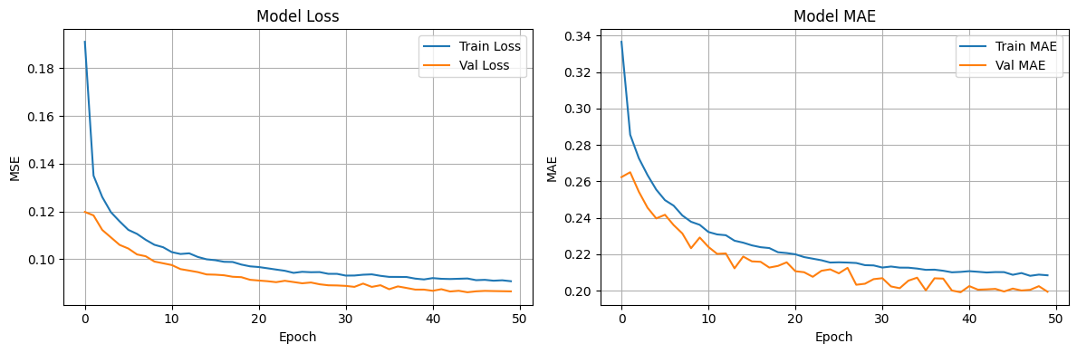
3. Conclusion
These values are expected.
y_pred = model.predict(X_test)

y_pred_steering = np.tanh(y_pred[:, 0])  # Steering: -1 to 1
y_pred_throttle = np.clip(y_pred[:, 1], 0, 1)  # Throttle: 0 to 1

y_pred_final = np.column_stack([y_pred_steering, y_pred_throttle])

steering_mae = np.mean(np.abs(y_test[:, 0] - y_pred_final[:, 0]))
throttle_mae = np.mean(np.abs(y_test[:, 1] - y_pred_final[:, 1]))

print(f"Steering MAE: {steering_mae:.4f}")
print(f"Throttle MAE: {throttle_mae:.4f}")
[1m173/173[0m [32m━━━━━━━━━━━━━━━━━━━━[0m[37m[0m [1m0s[0m 1ms/step
Steering MAE: 0.2397
Throttle MAE: 0.1614
plt.figure(figsize=(12, 4))

plt.subplot(1, 2, 1)
plt.plot(history.history['loss'], label='Train Loss')
plt.plot(history.history['val_loss'], label='Val Loss')
plt.title('Model Loss')
plt.xlabel('Epoch')
plt.ylabel('MSE')
plt.legend()
plt.grid(True)

plt.subplot(1, 2, 2)
plt.plot(history.history['mae'], label='Train MAE')
plt.plot(history.history['val_mae'], label='Val MAE')
plt.title('Model MAE')
plt.xlabel('Epoch')
plt.ylabel('MAE')
plt.legend()
plt.grid(True)

plt.tight_layout()
plt.savefig('training_history.png')
plt.show()
model.save("model.keras")