OT-ICA_Methodology_Validation.ipynb
Optimal Transport in linear Independent Component Analysis (ICA)
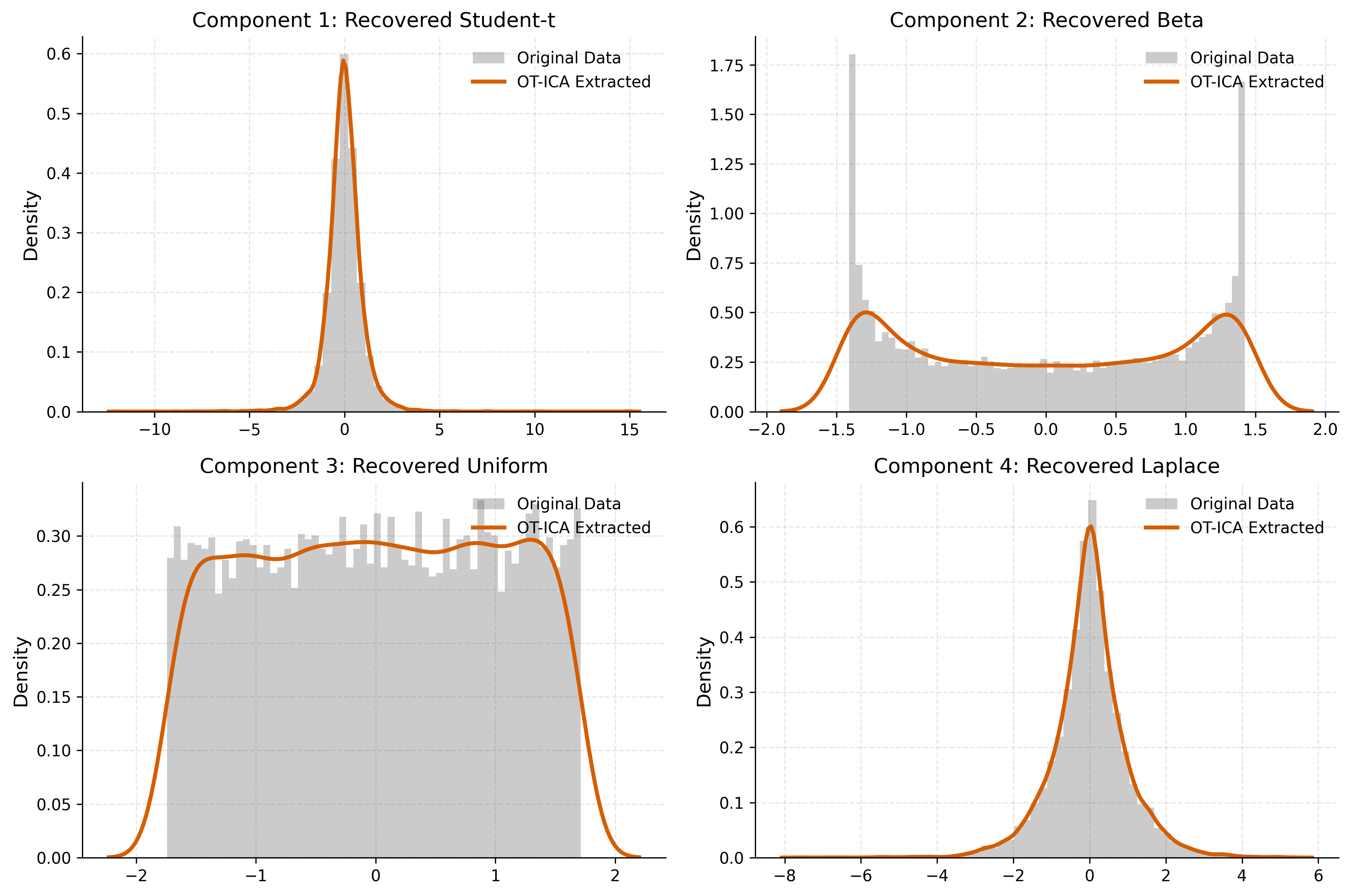
Here, We validate OT-ICA Methodology in a simple 4 dimensional case of ICA.
import numpy as np
import torch
import pandas as pd
import scipy.stats
import matplotlib.pyplot as plt
import matplotlib as mpl
import seaborn as sns
from sklearn.decomposition import FastICA
import warnings
from sklearn.exceptions import ConvergenceWarning

from wasserstein_ica import WassersteinICA
# Define a consistent Thesis Theme
def set_thesis_theme():
    # Academic, colorblind-friendly palette
    # Blue, Orange, Green, Red, Purple, Brown
    thesis_colors = ['#0173B2', '#DE8F05', '#029E73', '#D55E00', '#CC78BC', '#CA9161']

    mpl.rcParams.update({
        # Figure and Layout
        'figure.figsize': (8, 5),
        'figure.dpi': 300,            # High resolution for print
        'axes.prop_cycle': mpl.cycler(color=thesis_colors),

        # Grid lines (light and unobtrusive)
        'axes.grid': True,
        'grid.alpha': 0.3,
        'grid.linestyle': '--',
        'axes.axisbelow': True,       # Grid goes behind data

        # Spines (remove top and right borders for a cleaner look)
        'axes.spines.top': False,
        'axes.spines.right': False,

        # Fonts and Text
        'font.size': 11,
        'axes.titlesize': 13,
        'axes.labelsize': 12,
        'xtick.labelsize': 10,
        'ytick.labelsize': 10,

        # Legends
        'legend.frameon': False,      # No box around the legend
        'legend.fontsize': 10,

        # Lines
        'lines.linewidth': 2.0
    })

# Run this before plotting
set_thesis_theme()
def amari_error(W_est, A_true):
    if W_est is None or np.any(np.isnan(W_est)):
        return np.nan
    P = np.abs(W_est @ A_true)
    n = P.shape[0]
    row_sum = np.sum(P, axis=1)
    row_max = np.max(P, axis=1)
    term1 = np.sum((row_sum / row_max) - 1)
    col_sum = np.sum(P, axis=0)
    col_max = np.max(P, axis=0)
    term2 = np.sum((col_sum / col_max) - 1)
    return (term1 + term2) / (2 * n)
# ==========================================
# 1. Simulation Setup (4 Dimensions)
# ==========================================
n_samples = 10000
n_sources = 4
np.random.seed(42)
torch.manual_seed(42)

# Source 1: Laplace (Super-Gaussian, sharp peak)
s1 = np.random.laplace(0, 1, n_samples)
# Source 2: Uniform (Sub-Gaussian, flat)
s2 = np.random.uniform(-np.sqrt(3), np.sqrt(3), n_samples)
# Source 3: Student-t (Heavy tails, df=3)
s3 = np.random.standard_t(df=3, size=n_samples)
# Source 4: Beta(0.5, 0.5) (U-shaped, Bimodal)
s4 = np.random.beta(0.5, 0.5, size=n_samples)

# Stack, Center, and Normalize
S_true = np.stack([s1, s2, s3, s4])
S_true = (S_true - np.mean(S_true, axis=1, keepdims=True)) / np.std(S_true, axis=1, keepdims=True)
source_names = ['Laplace', 'Uniform', 'Student-t', 'Beta']

# Random well-conditioned Mixing Matrix
A_true = np.random.randn(n_sources, n_sources)
while np.linalg.cond(A_true) > 20:
    A_true = np.random.randn(n_sources, n_sources)

X_mixed = A_true @ S_true
X_torch = torch.tensor(X_mixed, dtype=torch.float32)

print("--- Ground Truth Mixing Matrix (A) ---")
print(np.round(A_true, 3))
--- Ground Truth Mixing Matrix (A) ---
[[ 1.058  1.52  -0.249  1.012]
 [ 0.042 -0.486  0.388 -0.523]
 [-0.154 -1.572 -0.304 -1.234]
 [-0.006  0.503  0.053  0.928]]
# ==========================================
# 2. Wasserstein ICA Extraction (Stiefel)
# ==========================================
print("\n--- Running W2-ICA ---")
device = torch.device('cuda' if torch.cuda.is_available() else 'cpu')
ica = WassersteinICA(X_torch.to(device))
ica.whiten()
W_white_np = ica.W_white.cpu().numpy()

# 2.1 Deflation Initialization
extracted_ws = []
for i in range(n_sources):
    prev = torch.stack(extracted_ws) if extracted_ws else None
    w, _ = ica.optimize_wasserstein2(
        prev_components=prev,
        max_iter=200,
        n_restarts=50,
        dither_sigma=0.01 # Crucial for Bernoulli
    )
    extracted_ws.append(w)

W_deflation_init = torch.stack(extracted_ws)

# 2.2 Symmetric Stiefel Polish
W_stiefel_unmixed = ica.optimize_symmetric(
    n_components=n_sources,
    max_iter=400,
    lr=0.25,
    init_w=W_deflation_init,
    optimizer='stiefel',
    dither_sigma=0.01,
    batch_size=1024
)

W_wass_total = W_stiefel_unmixed.cpu().numpy() @ W_white_np
score_wass = amari_error(W_wass_total, A_true)

print("\n--- Estimated Unmixing Matrix (W_est) ---")
print(np.round(W_wass_total, 3))
print(f"\nW2-ICA Amari Error: {score_wass:.5f}")
--- Running W2-ICA ---

--- Estimated Unmixing Matrix (W_est) ---
[[ 0.154 -1.943  0.608 -0.456]
 [-0.092 -0.284 -0.632 -1.977]
 [ 0.146  0.719  1.097  1.691]
 [ 1.021  1.204  0.828  0.677]]

W2-ICA Amari Error: 0.01552
# ==========================================
# 3. Source Matching
# ==========================================
# Global Transfer Matrix P = W_est @ A_true
P = W_wass_total @ A_true
print("\n--- Global Transfer Matrix (P) ---")
print(np.round(P, 3))

matches = []
for i in range(n_sources):
    row_abs = np.abs(P[i])
    best_match_idx = np.argmax(row_abs)
    sign = np.sign(P[i, best_match_idx])
    matches.append({
        "extracted_idx": i,
        "original_idx": best_match_idx,
        "name": source_names[best_match_idx],
        "sign": sign
    })
--- Global Transfer Matrix (P) ---
[[-0.01  -0.007 -1.    -0.002]
 [ 0.    -0.003  0.    -1.   ]
 [ 0.006 -1.    -0.002 -0.012]
 [ 1.     0.006 -0.003  0.01 ]]
# Extract Signals
Y_est = W_wass_total @ X_mixed

# ==========================================
# 4. Visualization
# ==========================================
fig, axes = plt.subplots(2, 2, figsize=(12, 8))
axes = axes.flatten()

for m in matches:
    i = m['extracted_idx']
    j = m['original_idx']
    sign = m['sign']

    orig = S_true[j]
    est = Y_est[i] * sign # Fix sign flip

    ax = axes[i]

    # Gray Histogram Bars for Original Data (No shading)
    ax.hist(orig, bins=60, density=True, alpha=0.3, color='#555555', edgecolor='none', label='Original Data')
    # Sharp Orange Line for Extracted Data
    sns.kdeplot(est, ax=ax, color='#D55E00', linewidth=2.5, label='OT-ICA Extracted')

    ax.set_title(f"Component {i+1}: Recovered {m['name']}", fontsize=13)
    ax.legend(loc='upper right', fontsize=10)

plt.tight_layout()
#plt.savefig('otica_baseline_recovery.png', dpi=300, bbox_inches='tight')
plt.show()
Comparison: Wasserstein versus FAST ICA using Amari Similarity measure
- P = U.M, where U is unmixing and M is mixing matrix and P should ideally have only one non zero entry per row
The Formula $$ E_{Amari} = \frac{1}{2n(n-1)} \left[ \sum_{i=1}^{n} \left( \frac{\sum_{j=1}^{n} |g_{ij}|}{\max_j |g_{ij}|} - 1 \right) + \sum_{j=1}^{n} \left( \frac{\sum_{i=1}^{n} |g_{ij}|}{\max_i |g_{ij}|} - 1 \right) \right] $$
Simon's Correction $$ E_{Amari} = \frac{1}{2n} \left[ \sum_{i=1}^{n} \left( \frac{\sum_{j=1}^{n} |g_{ij}|}{\max_j |g_{ij}|} - 1 \right) + \sum_{j=1}^{n} \left( \frac{\sum_{i=1}^{n} |g_{ij}|}{\max_i |g_{ij}|} - 1 \right) \right] $$
Interpretation
- 0.0: Perfect Separation (The matrices match exactly up to permutation/scale).
- < 0.4: Good/Acceptable Separation.
- > 0.5: Poor Separation (Failed to unmix).
from sklearn.decomposition import FastICA


# ==========================================
# 4. Method 2: FastICA (sklearn)
# ==========================================
print("\n--- Running FastICA (sklearn) ---")
# FastICA expects shape (n_samples, n_features)
X_sklearn = X_mixed.T

# Algorithm 1: Parallel FastICA with logcosh (approx Negentropy)
fastica = FastICA(n_components=n_sources, algorithm='parallel', fun='logcosh', random_state=42)
S_est_fast = fastica.fit_transform(X_sklearn)
W_total_fastica = fastica.components_ #@ fastica.whitening_ # Total unmixing matrix

score_fastica = amari_error(W_total_fastica, A_true)
print(f"FastICA (logcosh) Amari Error: {score_fastica:.5f}")
--- Running FastICA (sklearn) ---
FastICA (logcosh) Amari Error: 0.01879