Optimal Transport in linear ICA applied to Econometrics

In this application we test our methodology to find ICs in a simulated price discovery case between distinct markets

import numpy as np
import torch
import scipy.stats
import matplotlib.pyplot as plt
from scipy.optimize import linear_sum_assignment

from wasserstein_ica import WassersteinICA

import matplotlib.pyplot as plt
import matplotlib as mpl

# Define a consistent Thesis Theme
def set_thesis_theme():
    # Academic, colorblind-friendly palette
    # Blue, Orange, Green, Red, Purple, Brown
    thesis_colors = ['#0173B2', '#DE8F05', '#029E73', '#D55E00', '#CC78BC', '#CA9161']
    
    mpl.rcParams.update({
        # Figure and Layout
        'figure.figsize': (8, 5),
        'figure.dpi': 300,            # High resolution for print
        'axes.prop_cycle': mpl.cycler(color=thesis_colors),
        
        # Grid lines (light and unobtrusive)
        'axes.grid': True,
        'grid.alpha': 0.3,
        'grid.linestyle': '--',
        'axes.axisbelow': True,       # Grid goes behind data
        
        # Spines (remove top and right borders for a cleaner look)
        'axes.spines.top': False,
        'axes.spines.right': False,
        
        # Fonts and Text
        'font.size': 11,
        'axes.titlesize': 13,
        'axes.labelsize': 12,
        'xtick.labelsize': 10,
        'ytick.labelsize': 10,
        
        # Legends
        'legend.frameon': False,      # No box around the legend
        'legend.fontsize': 10,
        
        # Lines
        'lines.linewidth': 2.0
    })

# Run this before plotting
set_thesis_theme()

def apply_economic_constraints(W_est, W_white):
    """
    Post-process the statistical ICA output to enforce economic meaning.
    
    Addresses the critique that standard ICA results are permutation/sign indefinite.
    We apply:
    1. Dominant Diagonal: The shock impacting Market i the most is labeled Shock i.
    2. Positive Spillover: Structural shocks are normalized to have positive effects.
    
    Args:
        W_est (Torch Tensor): Unmixing matrix from ICA (Whitened space).
        W_white (Torch Tensor): Whitening matrix used.
        
    Returns:
        B_identified (Numpy Array): The economically identified Mixing Matrix.
    """
    # 1. Recover the Raw Mixing Matrix (B_raw)
    # The total estimated unmixing is W_tot = W_est @ W_white
    # The mixing matrix B is the inverse: X = B * S
    W_total = torch.matmul(W_est, W_white)
    B_raw = torch.linalg.inv(W_total).cpu().numpy()
    
    # 2. Permutation Constraint (Dominant Diagonal)
    # We use the Hungarian Algorithm (linear_sum_assignment) to match 
    # Shocks (columns) to Markets (rows) such that the diagonal magnitude is maximized.
    # We pass negative absolute values because the algorithm minimizes cost.
    row_ind, col_ind = linear_sum_assignment(-np.abs(B_raw))
    
    # Reorder the columns (shocks) of B
    B_permuted = B_raw[:, col_ind]
    
    # 3. Sign Constraint (Positive Impact)
    # Ensure the diagonal elements are positive (B_ii > 0).
    # If B_ii is negative, we assume we found the "negative" shock and flip the column.
    diagonals = np.diag(B_permuted)
    sign_corrections = np.sign(diagonals)
    
    # Broadcast multiplication to flip columns where sign is negative
    B_identified = B_permuted * sign_corrections[np.newaxis, :]
    
    return B_identified

# ==============================================================================
# EXPERIMENT SETUP (Replicating Zema & Cordoni DGP)
# ==============================================================================

# Simulation Settings
N_SIMULATIONS = 500       # Number of Monte Carlo runs
T_SAMPLES = 5000          # Observations per run (Daily returns)
N_MARKETS = 3
DEVICE = torch.device("cuda" if torch.cuda.is_available() else "cpu")

# Define the "True" Structure
# We target Information Shares: [0.12, 0.24, 0.64]
# Assuming a standard VECM where the orthogonal complement to beta is [1, 1, 1],
# The IS is proportional to the squared column sums of B.
target_is = np.array([0.12, 0.24, 0.64])
psi = np.array([1.0, 1.0, 1.0]) # Long-run impact vector

# Construct a True Mixing Matrix B that yields these shares.
# For simplicity, we use a diagonal B scaled by sqrt(target).
# (Note: Even with a diagonal B_true, the ICA has to work because we whiten the data,
# effectively destroying the structure, and ICA must rotate it back).
B_true = np.diag(np.sqrt(target_is)) 

print(f"Running Experiment on {DEVICE}...")
print(f"Target True IS: {target_is}")
print(f"Constraint Mode: Dominant Diagonal & Positive Signs")

results_is = []

Running Experiment on cuda...
Target True IS: [0.12 0.24 0.64]
Constraint Mode: Dominant Diagonal & Positive Signs

for sim in range(N_SIMULATIONS):
    
    # --- A. Data Generation (Student-t Innovations) ---
    # Independent shocks with degrees of freedom 5, 6, 7 (Heavy tails)
    s1 = np.random.standard_t(df=5, size=T_SAMPLES)
    s2 = np.random.standard_t(df=6, size=T_SAMPLES)
    s3 = np.random.standard_t(df=7, size=T_SAMPLES)
    
    # Stack and Normalize to unit variance (Standard ICA assumption)
    S = np.vstack([s1, s2, s3])
    S = S / S.std(axis=1, keepdims=True)
    
    # Mix the signals
    X_np = B_true @ S
    X_torch = torch.tensor(X_np, dtype=torch.float32, device=DEVICE)
    
    # --- B. Wasserstein ICA ---
    model = WassersteinICA(X_torch)
    model.whiten()
    
    dim = X_torch.shape[0]
    num_restarts = min(dim * 4, 150)
    
    # 
    # OPTIMIZATION PHASE 1: Deflationary SGD
    # Sequentially extract components to form a robust initialization matrix
    W_init_list = []
    prev_components = torch.empty((0, dim), device=DEVICE)
    
    for k in range(dim):
        w_k, _ = model.optimize_wasserstein2(
            prev_components=prev_components,
            continuous=True,
            max_iter=200,
            lr=0.1,
            n_restarts=num_restarts
        )
        W_init_list.append(w_k)
        prev_components = torch.cat([prev_components, w_k.unsqueeze(0)], dim=0)
        
    W_init = torch.stack(W_init_list)
    
    # OPTIMIZATION PHASE 2: Symmetric Stiefel Optimization
    # Refine the initial matrix simultaneously on the Stiefel manifold
    W_opt = model.optimize_symmetric(
        n_components=dim,
        optimizer='stiefel',
        init_w=W_init,
        use_sinkhorn=False,
        max_iter=300,
        lr=1.0
    )
    
    # --- C. Economic Identification ---
    B_final = apply_economic_constraints(W_opt, model.W_white)
    
    # --- D. Calculate Information Share ---
    # Calculate the long-run impact of each shock: Psi * B_column
    # Since Psi=[1,1,1], this is just the column sum.
    impacts = psi @ B_final
    
    # Variance contribution = impact^2
    variances = impacts ** 2
    
    # Information Share = Variance / Total Variance
    estimated_is = variances / np.sum(variances)
    results_is.append(estimated_is)
    
    if (sim + 1) % 10 == 0:
        print(f"Simulation {sim+1}/{N_SIMULATIONS} completed.")

Simulation 10/500 completed.
Simulation 20/500 completed.
Simulation 30/500 completed.
Simulation 40/500 completed.
Simulation 50/500 completed.
Simulation 60/500 completed.
Simulation 70/500 completed.
Simulation 80/500 completed.
Simulation 90/500 completed.
Simulation 100/500 completed.
Simulation 110/500 completed.
Simulation 120/500 completed.
Simulation 130/500 completed.
Simulation 140/500 completed.
Simulation 150/500 completed.
Simulation 160/500 completed.
Simulation 170/500 completed.
Simulation 180/500 completed.
Simulation 190/500 completed.
Simulation 200/500 completed.
Simulation 210/500 completed.
Simulation 220/500 completed.
Simulation 230/500 completed.
Simulation 240/500 completed.
Simulation 250/500 completed.
Simulation 260/500 completed.
Simulation 270/500 completed.
Simulation 280/500 completed.
Simulation 290/500 completed.
Simulation 300/500 completed.
Simulation 310/500 completed.
Simulation 320/500 completed.
Simulation 330/500 completed.
Simulation 340/500 completed.
Simulation 350/500 completed.
Simulation 360/500 completed.
Simulation 370/500 completed.
Simulation 380/500 completed.
Simulation 390/500 completed.
Simulation 400/500 completed.
Simulation 410/500 completed.
Simulation 420/500 completed.
Simulation 430/500 completed.
Simulation 440/500 completed.
Simulation 450/500 completed.
Simulation 460/500 completed.
Simulation 470/500 completed.
Simulation 480/500 completed.
Simulation 490/500 completed.
Simulation 500/500 completed.

#==============================================================================
# RESULTS TABLE
# ==============================================================================
results_is = np.array(results_is)
mean_is = np.mean(results_is, axis=0)
std_is = np.std(results_is, axis=0)

print("\n" + "="*60)
print(f"{'Market / Source':<15} | {'True IS':<10} | {'Est. IS (Mean)':<15} | {'Std Dev':<10}")
print("-" * 60)

for i in range(N_MARKETS):
    print(f"Market {i+1:<14} | {target_is[i]:<10.4f} | {mean_is[i]:<15.4f} | {std_is[i]:<10.4f}")

print("="*60)

============================================================
Market / Source | True IS    | Est. IS (Mean)  | Std Dev   
------------------------------------------------------------
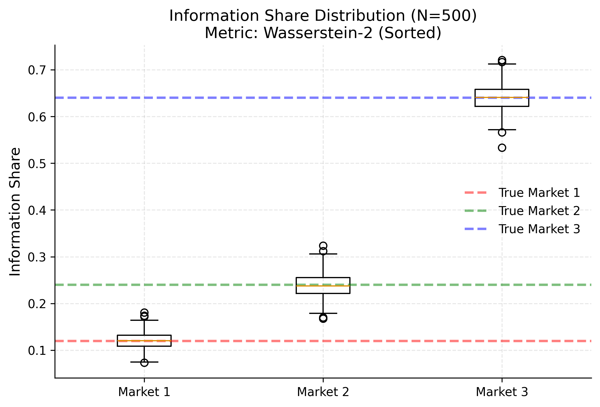
Market 1              | 0.1200     | 0.1212          | 0.0170    
Market 2              | 0.2400     | 0.2386          | 0.0249    
Market 3              | 0.6400     | 0.6402          | 0.0273    
============================================================

plt.figure(figsize=(8, 5))
plt.boxplot(results_is, tick_labels=['Market 1', 'Market 2', 'Market 3'])
plt.title(f"Information Share Distribution (N={N_SIMULATIONS})\nMetric: Wasserstein-2 (Sorted)")
plt.ylabel("Information Share")
# Draw True IS lines
colors = ['red', 'green', 'blue']
for i in range(3):
    plt.axhline(target_is[i], color=colors[i], linestyle='--', alpha=0.5, label=f'True Market {i+1}')
plt.legend()
plt.grid(True, alpha=0.3)
plt.show()

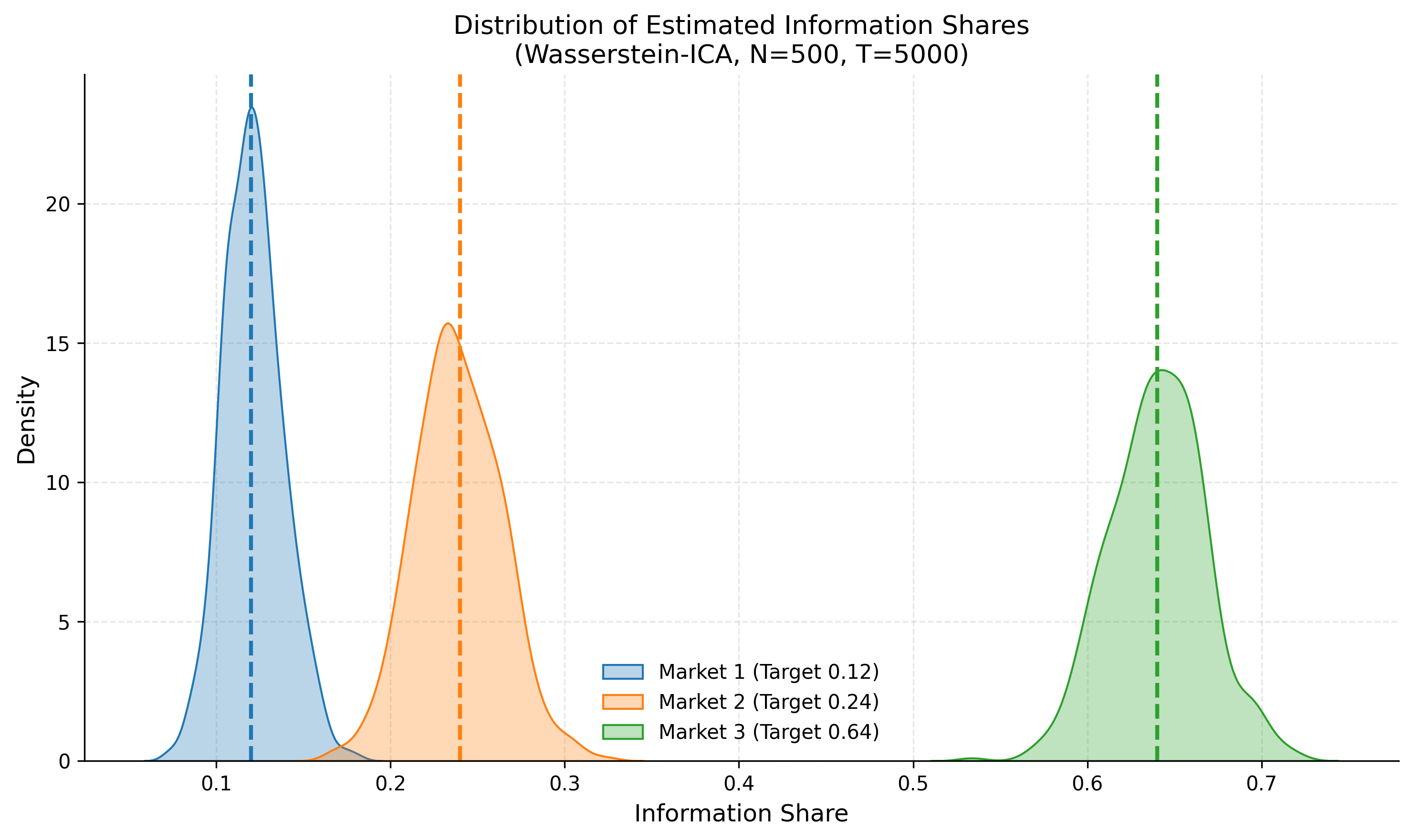
import matplotlib.pyplot as plt
import seaborn as sns # Optional, for nicer plots

# Plotting the distributions of Estimated Information Shares
plt.figure(figsize=(10, 6))

colors = ['#1f77b4', '#ff7f0e', '#2ca02c'] # Blue, Orange, Green
labels = ['Market 1 (Target 0.12)', 'Market 2 (Target 0.24)', 'Market 3 (Target 0.64)']
targets = [0.12, 0.24, 0.64]

for i in range(3):
    # Extract the column for Market i across all 500 simulations
    data = results_is[:, i]
    
    # Plot Histogram/KDE
    sns.kdeplot(data, color=colors[i], fill=True, alpha=0.3, label=labels[i])
    plt.axvline(targets[i], color=colors[i], linestyle='--', linewidth=2)

plt.title(f'Distribution of Estimated Information Shares\n(Wasserstein-ICA, N={N_SIMULATIONS}, T={T_SAMPLES})')
plt.xlabel('Information Share')
plt.ylabel('Density')
plt.legend()
plt.grid(True, alpha=0.3)
plt.tight_layout()
plt.show()

Economic Identification Strategy

Unlike the statistical output of raw ICA, which is permutation and sign indeterminate, we impose two strict economic constraints to recover the structural parameters:

1. Dominant Diagonal (Permutation): We strictly enforce that the structural shock assigned to Market $i$ must be the one that contributes the maximum variance to that specific market. This is implemented via the Hungarian Algorithm to solve the assignment problem.
2. Positive Impact (Sign): We assume positive spillovers, meaning a structural innovation (good news) must have a positive initial impact on its own price. Negative coefficients are sign-flipped.