OT_vs_FastICA_lbgfs.ipynb
Optimal Transport based ICA versus FastICA - linear setting
We compare the performance of OT based ICA and FastICA over varying number of dimensions and sample size of simulation with LBGFS optimization instead of SGD.
import numpy as np
import torch
import matplotlib.pyplot as plt
import pandas as pd
import seaborn as sns
from sklearn.decomposition import FastICA
from tqdm.notebook import tqdm

# IMPORT YOUR PACKAGE
from wasserstein_ica import WassersteinICA
# ==========================================
# 1. Metrics & Simulation Helpers
# ==========================================

def amari_error(W_est, A_true):
    """
    Computes the Amari Performance Index.
    0.0 = Perfect recovery (up to permutation/scale).
    """
    if W_est is None or np.any(np.isnan(W_est)):
        return np.nan

    P = np.abs(W_est @ A_true)
    n = P.shape[0]

    # Sum over rows
    row_sum = np.sum(P, axis=1)
    row_max = np.max(P, axis=1)
    term1 = np.sum((row_sum / row_max) - 1)

    # Sum over cols
    col_sum = np.sum(P, axis=0)
    col_max = np.max(P, axis=0)
    term2 = np.sum((col_sum / col_max) - 1)

    return (term1 + term2) / (2 * n)
def get_whitening_matrix(X_torch):
    """
    Helper to reconstruct the Whitening Matrix W_white used inside your class.
    We need this to calculate the Total Unmixing Matrix: W_total = W_sphere @ W_white
    """
    n_samples = X_torch.shape[1]
    X_centered = X_torch - torch.mean(X_torch, dim=1, keepdim=True)
    cov = torch.matmul(X_centered, X_centered.t()) / (n_samples - 1)
    D, E = torch.linalg.eigh(cov)
    D_inv_sqrt = torch.diag(1.0 / torch.sqrt(D + 1e-5))
    W = torch.matmul(D_inv_sqrt, E.T)
    return W.cpu().numpy()

def generate_dataset(n_dim, n_samples, seed=None, dist_type='laplace'):
    """
    Generates mixed data where ALL sources come from the same distribution family.

    Parameters:
    -----------
    dist_type : str
        'laplace'   (Super-Gaussian, sharp peak) - Standard ICA Benchmark
        'uniform'   (Sub-Gaussian, flat)         - Hard for some algorithms
        'student-t' (Heavy-tailed, df=3)         - Good for robustness check
        'beta'      (U-shaped, bimodal-ish)
    """
    if seed is not None:
        np.random.seed(seed)
        torch.manual_seed(seed)

    sources = []
    for _ in range(n_dim):
        if dist_type == 'laplace':
            # Standard Laplace (Mean=0, Scale=1)
            s = np.random.laplace(0, 1, n_samples)

        elif dist_type == 'uniform':
            # Unit variance Uniform [-sqrt(3), sqrt(3)]
            s = np.random.uniform(-np.sqrt(3), np.sqrt(3), n_samples)

        elif dist_type == 'student-t':
            # Heavy tails (Degrees of Freedom = 3)
            s = np.random.standard_t(df=3, size=n_samples)

        elif dist_type == 'beta':
            # Beta(0.5, 0.5) is "Arcsine" (U-shaped)
            s = np.random.beta(0.5, 0.5, size=n_samples)
            s = (s - np.mean(s)) / np.std(s) # Normalize

        else:
            raise ValueError(f"Unknown dist_type: {dist_type}")

        sources.append(s)

    S = np.stack(sources)

    # Random Mixing Matrix with condition number check
    cond_num = 1000
    while cond_num > 100:
        A = np.random.randn(n_dim, n_dim)
        cond_num = np.linalg.cond(A)

    X = A @ S
    return torch.tensor(X, dtype=torch.float32), A
# ==========================================
# 2. Experiment Configuration
# ==========================================

# --- Laptop Settings (Fast/Debug) ---
DIMENSION_RANGE = list(range(2, 36))      # Varying D
SAMPLE_SIZE_RANGE = [500, 1000, 5000] + list(range(10000, 100001, 5000)) # Varying N
N_TRIALS = 3                          # Repeats per point (for Error Bars)

# --- Cluster Settings---
# DIMENSION_RANGE = [2, 4, 8, 16, 32]
# SAMPLE_SIZE_RANGE = [500, 1000, 5000, 10000, 50000]
# N_TRIALS = 20

# Fixed Constants for the opposing experiment
FIXED_DIM = 6         # Used when varying Sample Size
FIXED_SAMPLES = 2000  # Used when varying Dimensions

print(f"--- Configuration ---")
print(f"Varying Dimensions: {DIMENSION_RANGE} (at N={FIXED_SAMPLES})")
print(f"Varying Samples:    {SAMPLE_SIZE_RANGE} (at D={FIXED_DIM})")
print(f"Trials per setting: {N_TRIALS}")
--- Configuration ---
Varying Dimensions: [2, 3, 4, 5, 6, 7, 8, 9, 10, 11, 12, 13, 14, 15, 16, 17, 18, 19, 20, 21, 22, 23, 24, 25, 26, 27, 28, 29, 30, 31, 32, 33, 34, 35] (at N=2000)
Varying Samples:    [500, 1000, 5000, 10000, 15000, 20000, 25000, 30000, 35000, 40000, 45000, 50000, 55000, 60000, 65000, 70000, 75000, 80000, 85000, 90000, 95000, 100000] (at D=6)
Trials per setting: 3
# ==========================================
# 3. Main Experiment Loop (L-BFGS Enabled)
# ==========================================
results = []

# --- Experiment A: Varying Dimensions ---
print("\nRunning Experiment 1: Varying Dimensions...")
for dim in tqdm(DIMENSION_RANGE, desc="Dimensions"):
    for trial in range(N_TRIALS):
        # 1. Data Gen
        X_torch, A_true = generate_dataset(n_dim=dim, n_samples=FIXED_SAMPLES, seed=trial, dist_type='laplace')
        X_np = X_torch.numpy()

        # 2. FastICA
        try:
            fast_ica = FastICA(n_components=dim, max_iter=2000, tol=1e-3, random_state=trial)
            fast_ica.fit(X_np.T)
            W_fast = fast_ica.components_
            score_fast = amari_error(W_fast, A_true)
        except Exception as e:
            score_fast = np.nan

        # 3. WassersteinICA (Deflation + L-BFGS Refinement)
        try:
            ica = WassersteinICA(X_torch)
            ica.whiten()

            # --- PHASE 1: Deflationary Initialization (Rough Draft with SGD) ---
            extracted_ws = []
            for _ in range(dim):
                prev = torch.stack(extracted_ws) if extracted_ws else None
                w, _ = ica.optimize_wasserstein2(
                    prev_components=prev,
                    max_iter=200,
                    lr=0.1,
                    continuous=True,
                    n_restarts=50
                )
                extracted_ws.append(w)

            W_deflation = torch.stack(extracted_ws)

            # --- PHASE 2: Symmetric Refinement (L-BFGS Polish) ---
            W_sphere = ica.optimize_symmetric(
                n_components=dim,
                init_w=W_deflation,
                max_iter=200,         # L-BFGS needs fewer iterations
                lr=1.0,              # Standard LR for L-BFGS
                optimizer='lbfgs',   # <--- ENABLE L-BFGS
                penalty_weight=10.0
            )

            # Reconstruct Total W
            W_white = get_whitening_matrix(X_torch)
            W_wass = W_sphere.cpu().numpy() @ W_white

            score_wass = amari_error(W_wass, A_true)
        except Exception as e:
            print(f"Wasserstein Fail (Dim {dim}): {e}")
            score_wass = np.nan

        results.append({'Exp': 'Varying Dim', 'X': dim, 'N': FIXED_SAMPLES, 'Method': 'FastICA', 'Amari': score_fast})
        results.append({'Exp': 'Varying Dim', 'X': dim, 'N': FIXED_SAMPLES, 'Method': 'WassersteinICA', 'Amari': score_wass})
Running Experiment 1: Varying Dimensions...


Dimensions:   0%|          | 0/34 [00:00<?, ?it/s]
# --- Experiment B: Varying Sample Size ---
print("\nRunning Experiment 2: Varying Sample Size...")
for n in tqdm(SAMPLE_SIZE_RANGE, desc="Samples"):
    for trial in range(N_TRIALS):
        # 1. Data Gen
        X_torch, A_true = generate_dataset(n_dim=FIXED_DIM, n_samples=n, seed=trial + 1000, dist_type='laplace')
        X_np = X_torch.numpy()

        # 2. FastICA
        try:
            fast_ica = FastICA(n_components=FIXED_DIM, max_iter=2000, tol=1e-3, random_state=trial)
            fast_ica.fit(X_np.T)
            W_fast = fast_ica.components_
            score_fast = amari_error(W_fast, A_true)
        except:
            score_fast = np.nan

        # 3. WassersteinICA
        try:
            ica = WassersteinICA(X_torch)
            ica.whiten()

            # Phase 1
            extracted_ws = []
            for _ in range(FIXED_DIM):
                prev = torch.stack(extracted_ws) if extracted_ws else None
                w, _ = ica.optimize_wasserstein2(
                    prev_components=prev,
                    max_iter=200,
                    lr=0.1,
                    continuous=True,
                    n_restarts=50
                )
                extracted_ws.append(w)

            W_deflation = torch.stack(extracted_ws)

            # Phase 2 (L-BFGS)
            W_sphere = ica.optimize_symmetric(
                n_components=FIXED_DIM,
                init_w=W_deflation,
                max_iter=200,
                lr=1.0,
                optimizer='lbfgs',
                penalty_weight=10.0
            )

            W_white = get_whitening_matrix(X_torch)
            W_wass = W_sphere.cpu().numpy() @ W_white

            score_wass = amari_error(W_wass, A_true)
        except Exception as e:
            print(f"Wasserstein Fail (N {n}): {e}")
            score_wass = np.nan

        results.append({'Exp': 'Varying N', 'X': n, 'N': n, 'Method': 'FastICA', 'Amari': score_fast})
        results.append({'Exp': 'Varying N', 'X': n, 'N': n, 'Method': 'WassersteinICA', 'Amari': score_wass})
Running Experiment 2: Varying Sample Size...


Samples:   0%|          | 0/22 [00:00<?, ?it/s]
df_results = pd.DataFrame(results)
# ==========================================
# 4A. Plotting Results: Varying Dimensions
# ==========================================
import seaborn as sns
import matplotlib.pyplot as plt
sns.set_style("whitegrid")
plt.figure(figsize=(8, 6))
# Filter Data for Dimensions Experiment
data_dim = df_results[df_results['Exp'] == 'Varying Dim']
# Plot
ax = sns.lineplot(
data=data_dim, x='X', y='Amari', hue='Method', style='Method',
markers=True, dashes=False, linewidth=2.5, errorbar=('ci', 95)
)
# Styling
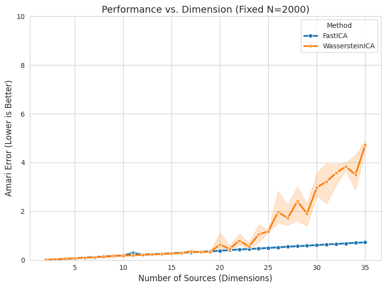
plt.title(f"Performance vs. Dimension (Fixed N={FIXED_SAMPLES})", fontsize=14)
plt.xlabel("Number of Sources (Dimensions)", fontsize=12)
plt.ylabel("Amari Error (Lower is Better)", fontsize=12)
plt.ylim(0, 10.0)
plt.tight_layout()
plt.show()
# Display Statistics Table for Dimensions
#print("\n--- Summary Statistics (Varying Dimensions) ---")
#display(data_dim.groupby(['X', 'Method'])['Amari'].agg(['mean', 'std']).round(4))
# ==========================================
# 4B. Plotting Results: Varying Sample Size
# ==========================================
import seaborn as sns
import matplotlib.pyplot as plt

sns.set_style("whitegrid")
plt.figure(figsize=(8, 6))

# Filter Data for Sample Size Experiment
data_n = df_results[df_results['Exp'] == 'Varying N']

# Plot
ax = sns.lineplot(
    data=data_n, x='X', y='Amari', hue='Method', style='Method',
    markers=True, dashes=False, linewidth=2.5, errorbar=('ci', 95)
)

# Styling
plt.title(f"Performance vs. Sample Size (Fixed D={FIXED_DIM})", fontsize=14)
plt.xlabel("Sample Size (N)", fontsize=12)
plt.xscale("log")  # Log scale is crucial for N
plt.ylabel("Amari Error (Lower is Better)", fontsize=12)
plt.ylim(0, 10.0)

plt.tight_layout()
plt.show()

# Display Statistics Table for Sample Size
print("\n--- Summary Statistics (Varying Sample Size) ---")
display(data_n.groupby(['X', 'Method'])['Amari'].agg(['mean', 'std']).round(4))
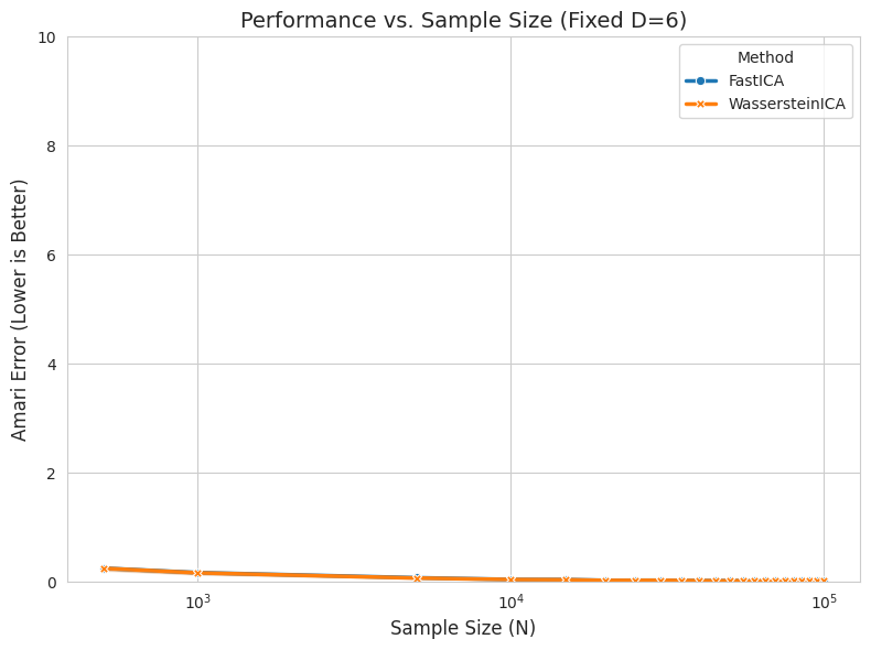
--- Summary Statistics (Varying Sample Size) ---
| mean | std | ||
|---|---|---|---|
| X | Method | ||
| 500 | FastICA | 0.2505 | 0.0270 |
| WassersteinICA | 0.2487 | 0.0376 | |
| 1000 | FastICA | 0.1695 | 0.0249 |
| WassersteinICA | 0.1653 | 0.0289 | |
| 5000 | FastICA | 0.0752 | 0.0117 |
| WassersteinICA | 0.0691 | 0.0108 | |
| 10000 | FastICA | 0.0435 | 0.0115 |
| WassersteinICA | 0.0422 | 0.0087 | |
| 15000 | FastICA | 0.0415 | 0.0016 |
| WassersteinICA | 0.0390 | 0.0029 | |
| 20000 | FastICA | 0.0271 | 0.0018 |
| WassersteinICA | 0.0260 | 0.0009 | |
| 25000 | FastICA | 0.0288 | 0.0040 |
| WassersteinICA | 0.0268 | 0.0041 | |
| 30000 | FastICA | 0.0290 | 0.0052 |
| WassersteinICA | 0.0273 | 0.0043 | |
| 35000 | FastICA | 0.0251 | 0.0055 |
| WassersteinICA | 0.0248 | 0.0061 | |
| 40000 | FastICA | 0.0228 | 0.0022 |
| WassersteinICA | 0.0218 | 0.0005 | |
| 45000 | FastICA | 0.0207 | 0.0019 |
| WassersteinICA | 0.0200 | 0.0028 | |
| 50000 | FastICA | 0.0203 | 0.0018 |
| WassersteinICA | 0.0195 | 0.0024 | |
| 55000 | FastICA | 0.0214 | 0.0011 |
| WassersteinICA | 0.0216 | 0.0004 | |
| 60000 | FastICA | 0.0163 | 0.0015 |
| WassersteinICA | 0.0152 | 0.0015 | |
| 65000 | FastICA | 0.0186 | 0.0017 |
| WassersteinICA | 0.0193 | 0.0025 | |
| 70000 | FastICA | 0.0182 | 0.0026 |
| WassersteinICA | 0.0178 | 0.0024 | |
| 75000 | FastICA | 0.0168 | 0.0006 |
| WassersteinICA | 0.0164 | 0.0004 | |
| 80000 | FastICA | 0.0163 | 0.0024 |
| WassersteinICA | 0.0150 | 0.0020 | |
| 85000 | FastICA | 0.0195 | 0.0040 |
| WassersteinICA | 0.0184 | 0.0032 | |
| 90000 | FastICA | 0.0167 | 0.0032 |
| WassersteinICA | 0.0166 | 0.0027 | |
| 95000 | FastICA | 0.0153 | 0.0013 |
| WassersteinICA | 0.0148 | 0.0009 | |
| 100000 | FastICA | 0.0138 | 0.0028 |
| WassersteinICA | 0.0128 | 0.0025 |
# ==========================================
# 5. Qualitative Analysis (L-BFGS Enabled)
# ==========================================
from scipy.optimize import linear_sum_assignment
def qualitative_check(n_dim=6, n_samples=2000):
print(f"\n--- Running Qualitative Check (Dim={n_dim}) ---")
# 1. Data Gen
X_torch, A_true = generate_dataset(n_dim=n_dim, n_samples=n_samples, seed=42, dist_type='laplace')
X_np = X_torch.numpy()
S_true = np.linalg.inv(A_true) @ X_np
# 2. Wasserstein ICA
ica = WassersteinICA(X_torch)
ica.whiten()
# Phase 1
extracted_ws = []
for _ in range(n_dim):
prev = torch.stack(extracted_ws) if extracted_ws else None
w, _ = ica.optimize_wasserstein2(
prev_components=prev, max_iter=200, lr=0.1, continuous=True, n_restarts=50
)
extracted_ws.append(w)
W_deflation = torch.stack(extracted_ws)
# Phase 2 (L-BFGS Polish)
W_sphere = ica.optimize_symmetric(
n_components=n_dim,
init_w=W_deflation,
max_iter=50,
lr=1.0,
optimizer='lbfgs',
penalty_weight=10.0
)
# Get Total W
W_white = get_whitening_matrix(X_torch)
W_est = W_sphere.cpu().numpy() @ W_white
S_est = W_est @ X_np
# 3. Match Sources
corr_mat = np.zeros((n_dim, n_dim))
for i in range(n_dim):
for j in range(n_dim):
corr_mat[i, j] = np.abs(np.corrcoef(S_true[i], S_est[j])[0, 1])
row_ind, col_ind = linear_sum_assignment(-corr_mat)
S_est_ordered = S_est[col_ind]
corr_mat_ordered = corr_mat[:, col_ind]
# 4. Global Matrix
P = np.abs(W_est @ A_true)
P_ordered = P[col_ind, :]
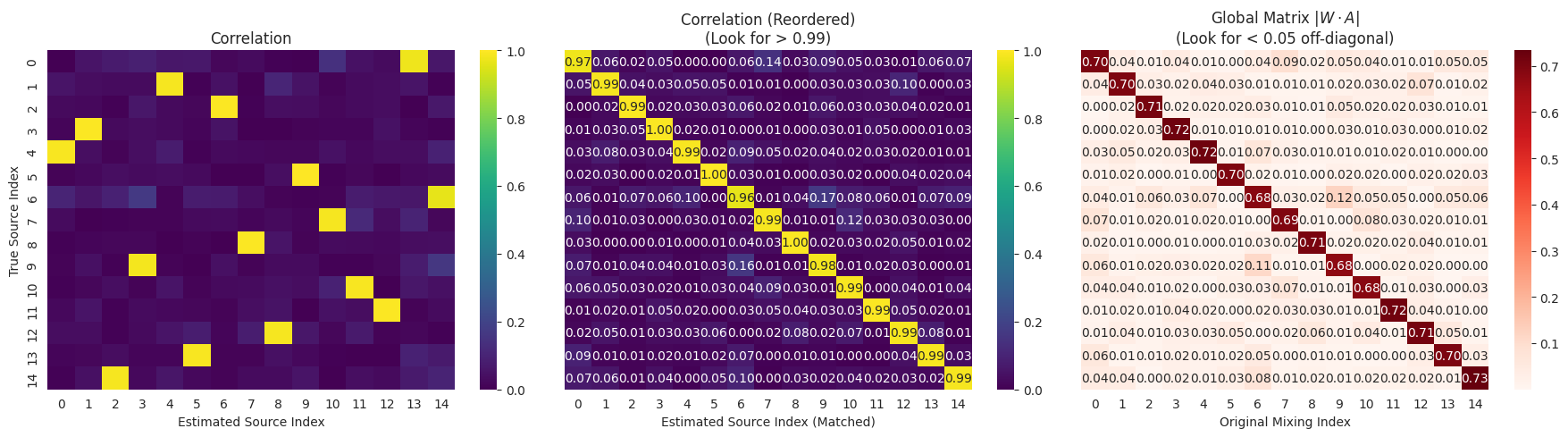
# Visuals
fig, axes = plt.subplots(1, 3, figsize=(18, 5))
sns.heatmap(corr_mat, ax=axes[0], cmap="viridis", vmin=0, vmax=1, annot=False)
axes[0].set_title("Correlation")
axes[0].set_xlabel("Estimated Source Index")
axes[0].set_ylabel("True Source Index")
sns.heatmap(corr_mat_ordered, ax=axes[1], cmap="viridis", vmin=0, vmax=1, annot=True, fmt=".2f")
axes[1].set_title("Correlation (Reordered)\n(Look for > 0.99)")
axes[1].set_xlabel("Estimated Source Index (Matched)")
axes[1].set_yticks([])
sns.heatmap(P_ordered, ax=axes[2], cmap="Reds", annot=True, fmt=".2f")
axes[2].set_title("Global Matrix $|W \\cdot A|$\n(Look for < 0.05 off-diagonal)")
axes[2].set_xlabel("Original Mixing Index")
axes[2].set_yticks([])
plt.tight_layout()
plt.show()
qualitative_check(n_dim=15)
--- Running Qualitative Check (Dim=15) ---