why_slow_OT_stiefel_ICA_over_FastICA.ipynb
Optimal Transport in linear ICA
In this notebook we present why anyone would use the slow OT Stiefel Manifold ICA (10 mins when dim=50, increases linearly with dimensions) over Fast ICA (<1 minute for dims=50).
Experiment: FastICA Contrast Functions vs. Wasserstein OT-ICA
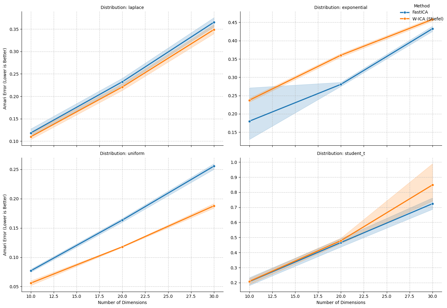
FastICA relies on scalar approximations (contrast functions like logcosh) that make specific geometric assumptions about the data. To demonstrate why the higher computational cost of Wasserstein OT-ICA (W-ICA) is justified, we test three distributions designed to expose the blind spots of parametric summaries:
- Exponential (The Asymmetric Blindspot): FastICA's default contrast functions are symmetric (even functions) and mathematically blind to skewness. W-ICA compares the entire Cumulative Distribution Function (CDF), natively capturing asymmetric geometry without needing to specify an odd moment.
- Student's t, df=7 (The Near-Gaussian Trap): Because it is very close to a perfect Gaussian, FastICA's moment approximations struggle to distinguish its subtle heavy tails from sample noise. W-ICA measures the exact volume of probability mass in the tails rather than relying on a summarized scalar.
- Uniform (The Hard Boundary): A sub-Gaussian distribution with negative kurtosis and absolute cutoffs. FastICA's continuous, smooth approximations struggle with sharp boundaries, whereas the Wasserstein metric natively maps flat geometries and bounded supports.
import numpy as np
import torch
import pandas as pd
import time
from sklearn.decomposition import FastICA
from joblib import Parallel, delayed
from tqdm.notebook import tqdm
from wasserstein_ica import WassersteinICA
# ==========================================
# 1. Helpers & Data Generation
# ==========================================

def amari_error(W_est, A_true):
    if W_est is None or np.any(np.isnan(W_est)):
        return np.nan

    P = np.abs(W_est @ A_true)
    n = P.shape[0]

    row_sum = np.sum(P, axis=1)
    row_max = np.max(P, axis=1)
    term1 = np.sum((row_sum / row_max) - 1)

    col_sum = np.sum(P, axis=0)
    col_max = np.max(P, axis=0)
    term2 = np.sum((col_sum / col_max) - 1)

    return (term1 + term2) / (2 * n)

def generate_dataset(n_dim, n_samples, dist_type='laplace', seed=None):
    if seed is not None:
        np.random.seed(seed)
        torch.manual_seed(seed)

    if dist_type == 'laplace':
        # Super-Gaussian, sharp peak
        sources = [np.random.laplace(0, 1, n_samples) for _ in range(n_dim)]
    elif dist_type == 'uniform':
        # Sub-Gaussian, bounded, negative kurtosis
        sources = [np.random.uniform(-np.sqrt(3), np.sqrt(3), n_samples) for _ in range(n_dim)]
    elif dist_type == 'exponential':
        # Highly skewed, asymmetric
        sources = [np.random.exponential(1.0, n_samples) - 1.0 for _ in range(n_dim)]
    elif dist_type == 'student_t':
        # Near-Gaussian, subtle heavy tails
        df = 7
        sources = [np.random.standard_t(df, n_samples) / np.sqrt(df / (df - 2)) for _ in range(n_dim)]
    else:
        raise ValueError("Unknown distribution type")

    S = np.stack(sources)

    # Well-conditioned mixing matrix
    cond_num = 1000
    while cond_num > 100:
        A = np.random.randn(n_dim, n_dim)
        cond_num = np.linalg.cond(A)

    X = A @ S
    return torch.tensor(X, dtype=torch.float32), A
# ==========================================
# 2. Parallel Worker Function
# ==========================================

def run_distribution_trial(dim, trial, n_samples, dist_type):
    torch.set_num_threads(1) # Prevent thread explosion
    trial_results = []

    X_torch, A_true = generate_dataset(n_dim=dim, n_samples=n_samples, dist_type=dist_type, seed=trial)
    X_np = X_torch.numpy()

    # --- FastICA ---
    t0_fast = time.perf_counter()
    try:
        fast_ica = FastICA(n_components=dim, max_iter=2000, tol=1e-4, random_state=trial)
        fast_ica.fit(X_np.T)
        W_fast_total = fast_ica.components_
        score_fast = amari_error(W_fast_total, A_true)
    except Exception:
        score_fast = np.nan
    t_fast_total = time.perf_counter() - t0_fast

    trial_results.append({
        'Distribution': dist_type,
        'Dimension': dim,
        'Method': 'FastICA',
        'Amari Error': score_fast,
        'Total Time (s)': t_fast_total
    })

    # --- W-ICA (Stiefel) ---
    t0_wass = time.perf_counter()
    try:
        ica = WassersteinICA(X_torch)
        ica.whiten()
        W_white_np = ica.W_white.cpu().numpy()

        extracted_ws = []
        n_restarts = dim * 4 if dim * 4 < 150 else 150
        for _ in range(dim):
            prev = torch.stack(extracted_ws) if extracted_ws else None
            w, _ = ica.optimize_wasserstein2(prev_components=prev, max_iter=200, n_restarts=n_restarts)
            extracted_ws.append(w)
        W_deflation_init = torch.stack(extracted_ws)

        W_stiefel_unmixed = ica.optimize_symmetric(
            n_components=dim, max_iter=200, lr=1.0, init_w=W_deflation_init, optimizer='stiefel'
        )
        W_wass_total = W_stiefel_unmixed.cpu().numpy() @ W_white_np
        score_wass = amari_error(W_wass_total, A_true)
    except Exception:
        score_wass = np.nan
    t_wass_total = time.perf_counter() - t0_wass

    trial_results.append({
        'Distribution': dist_type,
        'Dimension': dim,
        'Method': 'W-ICA (Stiefel)',
        'Amari Error': score_wass,
        'Total Time (s)': t_wass_total
    })

    return trial_results
# ==========================================
# 3. Main Execution
# ==========================================
DIMENSIONS = [10, 20, 30]
DISTRIBUTIONS = ['laplace', 'exponential', 'uniform', 'student_t_df_7']
N_SAMPLES = 5000
N_TRIALS = 5
tasks = [(dim, trial, N_SAMPLES, dist) for dist in DISTRIBUTIONS for dim in DIMENSIONS for trial in range(N_TRIALS)]

results_nested = Parallel(n_jobs=12)(
    delayed(run_distribution_trial)(dim, trial, n_samples, dist)
    for dim, trial, n_samples, dist in tqdm(tasks, desc="Running Multi-Dist Trials")
)

results = [item for sublist in results_nested for item in sublist]
df = pd.DataFrame(results)

# Display tabular summary
summary_table = df.groupby(['Distribution', 'Dimension', 'Method'])['Amari Error'].mean().unstack().round(4)
display(summary_table)
--- The Contrast Function Weakness Showdown ---


Running Multi-Dist Trials:   0%|          | 0/60 [00:00<?, ?it/s]
| Method | FastICA | W-ICA (Stiefel) | |
|---|---|---|---|
| Distribution | Dimension | ||
| exponential | 10 | 0.1800 | 0.2373 |
| 20 | 0.2806 | 0.3603 | |
| 30 | 0.4326 | 0.4580 | |
| laplace | 10 | 0.1183 | 0.1098 |
| 20 | 0.2324 | 0.2208 | |
| 30 | 0.3653 | 0.3489 | |
| student_t | 10 | 0.2070 | 0.2089 |
| 20 | 0.4665 | 0.4785 | |
| 30 | 0.7239 | 0.8484 | |
| uniform | 10 | 0.0769 | 0.0559 |
| 20 | 0.1635 | 0.1179 | |
| 30 | 0.2555 | 0.1877 |
import seaborn as sns
import matplotlib.pyplot as plt

# ==========================================
# 4. Multi-Distribution Visualization
# ==========================================

# 1. Pivot the data to get one mean Amari error per distribution, method, and dimension
# Seaborn's FacetGrid will automatically handle the trials/error bars

g = sns.FacetGrid(df, col="Distribution", col_wrap=2, height=5, aspect=1.3, sharey=False)

# 2. Map the lineplot to each facet.
# FacetGrid maps a standard seaborn lineplot (data=df, x=..., y=..., hue=...)
# while holding 'col' constant.
g.map_dataframe(
    sns.lineplot,
    x="Dimension",
    y="Amari Error",
    hue="Method",
    marker="o",
    linewidth=2.5
)

# 3. Titles and Labels
g.set_axis_labels("Number of Dimensions", "Amari Error (Lower is Better)")
g.set_titles("Distribution: {col_name}")

# 4. Format the graphs
for ax in g.axes.flat:
    ax.grid(True, linestyle='--', alpha=0.7)
    # Optional: Log scale helps see subtle differences near Gaussian
    # ax.set_yscale('log')

# 5. Add a single legend for the entire grid
g.add_legend(title="Method", loc='upper right')

plt.tight_layout()
plt.show()

# Display mean table one last time for context
display(df.groupby(['Distribution', 'Dimension', 'Method'])['Amari Error'].mean().unstack().round(4))
| Method | FastICA | W-ICA (Stiefel) | |
|---|---|---|---|
| Distribution | Dimension | ||
| exponential | 10 | 0.1800 | 0.2373 |
| 20 | 0.2806 | 0.3603 | |
| 30 | 0.4326 | 0.4580 | |
| laplace | 10 | 0.1183 | 0.1098 |
| 20 | 0.2324 | 0.2208 | |
| 30 | 0.3653 | 0.3489 | |
| student_t | 10 | 0.2070 | 0.2089 |
| 20 | 0.4665 | 0.4785 | |
| 30 | 0.7239 | 0.8484 | |
| uniform | 10 | 0.0769 | 0.0559 |
| 20 | 0.1635 | 0.1179 | |
| 30 | 0.2555 | 0.1877 |