
Finding How The Data Is Distributed
Estimated time needed: 30 minutes
In this lab, you will work with a cleaned dataset to perform Exploratory Data Analysis (EDA). You will examine the structure of the data, visualize key variables, and analyze trends related to developer experience, tools, job satisfaction, and other important aspects.
Objectives
In this lab you will perform the following:
-
Understand the structure of the dataset.
-
Perform summary statistics and data visualization.
-
Identify trends in developer experience, tools, job satisfaction, and other key variables.
Install the required libraries
!pip install pandas
!pip install matplotlib
!pip install seaborn
Requirement already satisfied: pandas in /opt/conda/lib/python3.12/site-packages (3.0.0)
Requirement already satisfied: numpy>=1.26.0 in /opt/conda/lib/python3.12/site-packages (from pandas) (2.4.1)
Requirement already satisfied: python-dateutil>=2.8.2 in /opt/conda/lib/python3.12/site-packages (from pandas) (2.9.0.post0)
Requirement already satisfied: six>=1.5 in /opt/conda/lib/python3.12/site-packages (from python-dateutil>=2.8.2->pandas) (1.17.0)
Requirement already satisfied: matplotlib in /opt/conda/lib/python3.12/site-packages (3.10.8)
Requirement already satisfied: contourpy>=1.0.1 in /opt/conda/lib/python3.12/site-packages (from matplotlib) (1.3.3)
Requirement already satisfied: cycler>=0.10 in /opt/conda/lib/python3.12/site-packages (from matplotlib) (0.12.1)
Requirement already satisfied: fonttools>=4.22.0 in /opt/conda/lib/python3.12/site-packages (from matplotlib) (4.61.1)
Requirement already satisfied: kiwisolver>=1.3.1 in /opt/conda/lib/python3.12/site-packages (from matplotlib) (1.4.9)
Requirement already satisfied: numpy>=1.23 in /opt/conda/lib/python3.12/site-packages (from matplotlib) (2.4.1)
Requirement already satisfied: packaging>=20.0 in /opt/conda/lib/python3.12/site-packages (from matplotlib) (24.2)
Requirement already satisfied: pillow>=8 in /opt/conda/lib/python3.12/site-packages (from matplotlib) (12.1.0)
Requirement already satisfied: pyparsing>=3 in /opt/conda/lib/python3.12/site-packages (from matplotlib) (3.3.2)
Requirement already satisfied: python-dateutil>=2.7 in /opt/conda/lib/python3.12/site-packages (from matplotlib) (2.9.0.post0)
Requirement already satisfied: six>=1.5 in /opt/conda/lib/python3.12/site-packages (from python-dateutil>=2.7->matplotlib) (1.17.0)
Requirement already satisfied: seaborn in /opt/conda/lib/python3.12/site-packages (0.13.2)
Requirement already satisfied: numpy!=1.24.0,>=1.20 in /opt/conda/lib/python3.12/site-packages (from seaborn) (2.4.1)
Requirement already satisfied: pandas>=1.2 in /opt/conda/lib/python3.12/site-packages (from seaborn) (3.0.0)
Requirement already satisfied: matplotlib!=3.6.1,>=3.4 in /opt/conda/lib/python3.12/site-packages (from seaborn) (3.10.8)
Requirement already satisfied: contourpy>=1.0.1 in /opt/conda/lib/python3.12/site-packages (from matplotlib!=3.6.1,>=3.4->seaborn) (1.3.3)
Requirement already satisfied: cycler>=0.10 in /opt/conda/lib/python3.12/site-packages (from matplotlib!=3.6.1,>=3.4->seaborn) (0.12.1)
Requirement already satisfied: fonttools>=4.22.0 in /opt/conda/lib/python3.12/site-packages (from matplotlib!=3.6.1,>=3.4->seaborn) (4.61.1)
Requirement already satisfied: kiwisolver>=1.3.1 in /opt/conda/lib/python3.12/site-packages (from matplotlib!=3.6.1,>=3.4->seaborn) (1.4.9)
Requirement already satisfied: packaging>=20.0 in /opt/conda/lib/python3.12/site-packages (from matplotlib!=3.6.1,>=3.4->seaborn) (24.2)
Requirement already satisfied: pillow>=8 in /opt/conda/lib/python3.12/site-packages (from matplotlib!=3.6.1,>=3.4->seaborn) (12.1.0)
Requirement already satisfied: pyparsing>=3 in /opt/conda/lib/python3.12/site-packages (from matplotlib!=3.6.1,>=3.4->seaborn) (3.3.2)
Requirement already satisfied: python-dateutil>=2.7 in /opt/conda/lib/python3.12/site-packages (from matplotlib!=3.6.1,>=3.4->seaborn) (2.9.0.post0)
Requirement already satisfied: six>=1.5 in /opt/conda/lib/python3.12/site-packages (from python-dateutil>=2.7->matplotlib!=3.6.1,>=3.4->seaborn) (1.17.0)
Step 1: Import Libraries and Load Data
-
Import the
pandas,matplotlib.pyplot, andseabornlibraries. -
You will begin with loading the dataset. You can use the pyfetch method if working on JupyterLite. Otherwise, you can use pandas' read_csv() function directly on their local machines or cloud environments.
# Import necessary libraries
import pandas as pd
import numpy as np
import matplotlib.pyplot as plt
import seaborn as sns
import textwrap

# Load the Stack Overflow survey dataset
data_url = 'https://cf-courses-data.s3.us.cloud-object-storage.appdomain.cloud/n01PQ9pSmiRX6520flujwQ/survey-data.csv'
df = pd.read_csv(data_url)

# Display the first few rows of the dataset
print(df.head())
print('Initial dataframe:', df.shape)
   ResponseId                      MainBranch                 Age  \
0           1  I am a developer by profession  Under 18 years old
1           2  I am a developer by profession     35-44 years old
2           3  I am a developer by profession     45-54 years old
3           4           I am learning to code     18-24 years old
4           5  I am a developer by profession     18-24 years old

            Employment RemoteWork   Check  \
0  Employed, full-time     Remote  Apples
1  Employed, full-time     Remote  Apples
2  Employed, full-time     Remote  Apples
3   Student, full-time        NaN  Apples
4   Student, full-time        NaN  Apples

                                    CodingActivities  \
0                                              Hobby
1  Hobby;Contribute to open-source projects;Other...
2  Hobby;Contribute to open-source projects;Other...
3                                                NaN
4                                                NaN

                                             EdLevel  \
0                          Primary/elementary school
1       Bachelor’s degree (B.A., B.S., B.Eng., etc.)
2    Master’s degree (M.A., M.S., M.Eng., MBA, etc.)
3  Some college/university study without earning ...
4  Secondary school (e.g. American high school, G...

                                           LearnCode  \
0                             Books / Physical media
1  Books / Physical media;Colleague;On the job tr...
2  Books / Physical media;Colleague;On the job tr...
3  Other online resources (e.g., videos, blogs, f...
4  Other online resources (e.g., videos, blogs, f...

                                     LearnCodeOnline  ... JobSatPoints_6  \
0                                                NaN  ...            NaN
1  Technical documentation;Blogs;Books;Written Tu...  ...            0.0
2  Technical documentation;Blogs;Books;Written Tu...  ...            NaN
3  Stack Overflow;How-to videos;Interactive tutorial  ...            NaN
4  Technical documentation;Blogs;Written Tutorial...  ...            NaN

  JobSatPoints_7 JobSatPoints_8 JobSatPoints_9 JobSatPoints_10  \
0            NaN            NaN            NaN             NaN
1            0.0            0.0            0.0             0.0
2            NaN            NaN            NaN             NaN
3            NaN            NaN            NaN             NaN
4            NaN            NaN            NaN             NaN

  JobSatPoints_11           SurveyLength SurveyEase ConvertedCompYearly JobSat
0             NaN                    NaN        NaN                 NaN    NaN
1             0.0                    NaN        NaN                 NaN    NaN
2             NaN  Appropriate in length       Easy                 NaN    NaN
3             NaN               Too long       Easy                 NaN    NaN
4             NaN              Too short       Easy                 NaN    NaN

[5 rows x 114 columns]
Initial dataframe: (65437, 114)
Step 2: Examine the Structure of the Data
-
Display the column names, data types, and summary information to understand the data structure.
-
Objective: Gain insights into the dataset's shape and available variables.
## Write your code here
print(df.dtypes.sort_index().to_string())
print(df.info())
AIAcc                                 str
AIBen                                 str
AIChallenges                          str
AIComplex                             str
AIEthics                              str
AINextLess integrated                 str
AINextMore integrated                 str
AINextMuch less integrated            str
AINextMuch more integrated            str
AINextNo change                       str
AISearchDevAdmired                    str
AISearchDevHaveWorkedWith             str
AISearchDevWantToWorkWith             str
AISelect                              str
AISent                                str
AIThreat                              str
AIToolCurrently Using                 str
AIToolInterested in Using             str
AIToolNot interested in Using         str
Age                                   str
BuildvsBuy                            str
BuyNewTool                            str
Check                                 str
CodingActivities                      str
CompTotal                         float64
ConvertedCompYearly               float64
Country                               str
Currency                              str
DatabaseAdmired                       str
DatabaseHaveWorkedWith                str
DatabaseWantToWorkWith                str
DevType                               str
EdLevel                               str
EmbeddedAdmired                       str
EmbeddedHaveWorkedWith                str
EmbeddedWantToWorkWith                str
Employment                            str
Frequency_1                           str
Frequency_2                           str
Frequency_3                           str
Frustration                           str
ICorPM                                str
Industry                              str
JobSat                            float64
JobSatPoints_1                    float64
JobSatPoints_10                   float64
JobSatPoints_11                   float64
JobSatPoints_4                    float64
JobSatPoints_5                    float64
JobSatPoints_6                    float64
JobSatPoints_7                    float64
JobSatPoints_8                    float64
JobSatPoints_9                    float64
Knowledge_1                           str
Knowledge_2                           str
Knowledge_3                           str
Knowledge_4                           str
Knowledge_5                           str
Knowledge_6                           str
Knowledge_7                           str
Knowledge_8                           str
Knowledge_9                           str
LanguageAdmired                       str
LanguageHaveWorkedWith                str
LanguageWantToWorkWith                str
LearnCode                             str
LearnCodeOnline                       str
MainBranch                            str
MiscTechAdmired                       str
MiscTechHaveWorkedWith                str
MiscTechWantToWorkWith                str
NEWCollabToolsAdmired                 str
NEWCollabToolsHaveWorkedWith          str
NEWCollabToolsWantToWorkWith          str
NEWSOSites                            str
OfficeStackAsyncAdmired               str
OfficeStackAsyncHaveWorkedWith        str
OfficeStackAsyncWantToWorkWith        str
OfficeStackSyncAdmired                str
OfficeStackSyncHaveWorkedWith         str
OfficeStackSyncWantToWorkWith         str
OpSysPersonal use                     str
OpSysProfessional use                 str
OrgSize                               str
PlatformAdmired                       str
PlatformHaveWorkedWith                str
PlatformWantToWorkWith                str
ProfessionalCloud                     str
ProfessionalQuestion                  str
ProfessionalTech                      str
PurchaseInfluence                     str
RemoteWork                            str
ResponseId                          int64
SOAccount                             str
SOComm                                str
SOHow                                 str
SOPartFreq                            str
SOVisitFreq                           str
SurveyEase                            str
SurveyLength                          str
TBranch                               str
TechDoc                               str
TechEndorse                           str
TimeAnswering                         str
TimeSearching                         str
ToolsTechAdmired                      str
ToolsTechHaveWorkedWith               str
ToolsTechWantToWorkWith               str
WebframeAdmired                       str
WebframeHaveWorkedWith                str
WebframeWantToWorkWith                str
WorkExp                           float64
YearsCode                             str
YearsCodePro                          str
<class 'pandas.DataFrame'>
RangeIndex: 65437 entries, 0 to 65436
Columns: 114 entries, ResponseId to JobSat
dtypes: float64(13), int64(1), str(100)
memory usage: 56.9 MB
None
Step 3: Handle Missing Data
-
Identify missing values in the dataset.
-
Impute or remove missing values as necessary to ensure data completeness.
## Write your code here
frnan = df.isna().mean().sort_values(ascending=False).round(decimals=4)
print('Fraction of missing values in each column')
print(frnan.head())
Fraction of missing values in each column
AINextMuch less integrated    0.9825
AINextLess integrated         0.9640
AINextNo change               0.8090
AINextMuch more integrated    0.7946
EmbeddedAdmired               0.7443
dtype: float64
# Drop the rows where all elements are missing.
df_m = df.dropna(how="all")
print('Initial dataframe:', df.shape)
print('Modified dataframe:', df_m.shape)
Initial dataframe: (65437, 114)
Modified dataframe: (65437, 114)
Step 4: Analyze Key Columns
-
Examine key columns such as
Employment,JobSat(Job Satisfaction), andYearsCodePro(Professional Coding Experience). -
Instruction: Calculate the value counts for each column to understand the distribution of responses.
## Write your code here
keycol = ['Employment', 'JobSat', 'YearsCodePro']
for col in keycol:
    print(df_m[col].value_counts(), '\n')
Employment
Employed, full-time                                                                                                                                   39041
Independent contractor, freelancer, or self-employed                                                                                                   4846
Student, full-time                                                                                                                                     4709
Employed, full-time;Independent contractor, freelancer, or self-employed                                                                               3557
Not employed, but looking for work                                                                                                                     2341
                                                                                                                                                      ...
Not employed, but looking for work;Independent contractor, freelancer, or self-employed;Not employed, and not looking for work;Employed, part-time        1
Student, full-time;Retired                                                                                                                                1
Employed, full-time;Not employed, but looking for work;Student, part-time                                                                                 1
Not employed, and not looking for work;Student, part-time;Employed, part-time                                                                             1
Not employed, but looking for work;Independent contractor, freelancer, or self-employed;Student, part-time;Retired                                        1
Name: count, Length: 110, dtype: int64

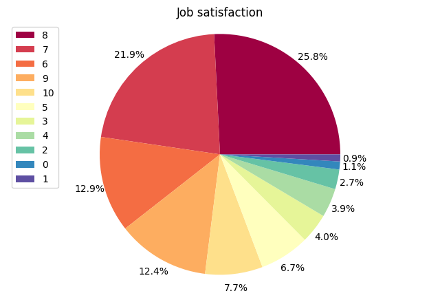
JobSat
8.0     7509
7.0     6379
6.0     3751
9.0     3626
10.0    2251
5.0     1956
3.0     1165
4.0     1130
2.0      772
0.0      311
1.0      276
Name: count, dtype: int64

YearsCodePro
2                     4168
3                     4093
5                     3526
10                    3251
4                     3215
Less than 1 year      2856
6                     2843
1                     2639
8                     2549
7                     2517
12                    1777
15                    1635
20                    1549
9                     1493
11                    1312
13                    1127
14                    1082
25                     998
16                     946
18                     867
17                     814
30                     689
24                     632
19                     516
22                     492
23                     448
26                     426
27                     380
21                     380
28                     342
35                     285
29                     196
32                     194
40                     194
34                     169
38                     134
33                     132
36                     119
31                     106
37                     104
45                      56
42                      55
39                      54
41                      51
More than 50 years      50
44                      42
43                      37
46                      21
50                      14
48                      14
49                      11
47                      10
Name: count, dtype: int64
Step 5: Visualize Job Satisfaction (Focus on JobSat)
-
Create a pie chart or KDE plot to visualize the distribution of
JobSat. -
Provide an interpretation of the plot, highlighting key trends in job satisfaction.
## Write your code here
JobSatpl = df_m.JobSat.value_counts()
JobSatpl.plot(kind='pie',
              figsize=(8, 5),
              autopct='%1.1f%%', # add in percentages
              labels=None,
              startangle=0,
              pctdistance=1.12,  # the ratio between the center of each pie slice and the start of the text
              shadow=False,
              colormap='Spectral'
              )

plt.title('Job satisfaction')
plt.axis('equal') # Sets the pie chart to look like a circle
plt.legend(labels=JobSatpl.index.astype(int), loc='upper left')

plt.show()
plt.figure(figsize=(8,5))
sns.kdeplot(data=df_m.JobSat, bw_adjust=0.3)
plt.title('Job satisfaction')
plt.grid(True, linestyle='dashed')
plt.xticks(range(0, 11, 1))
plt.ylabel('Proportion of answers')
plt.show()
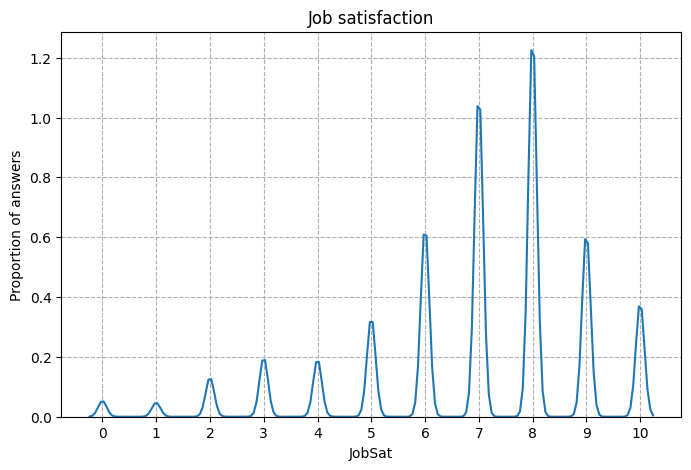
# Most of the people experienced job satisfaction higher than 5.
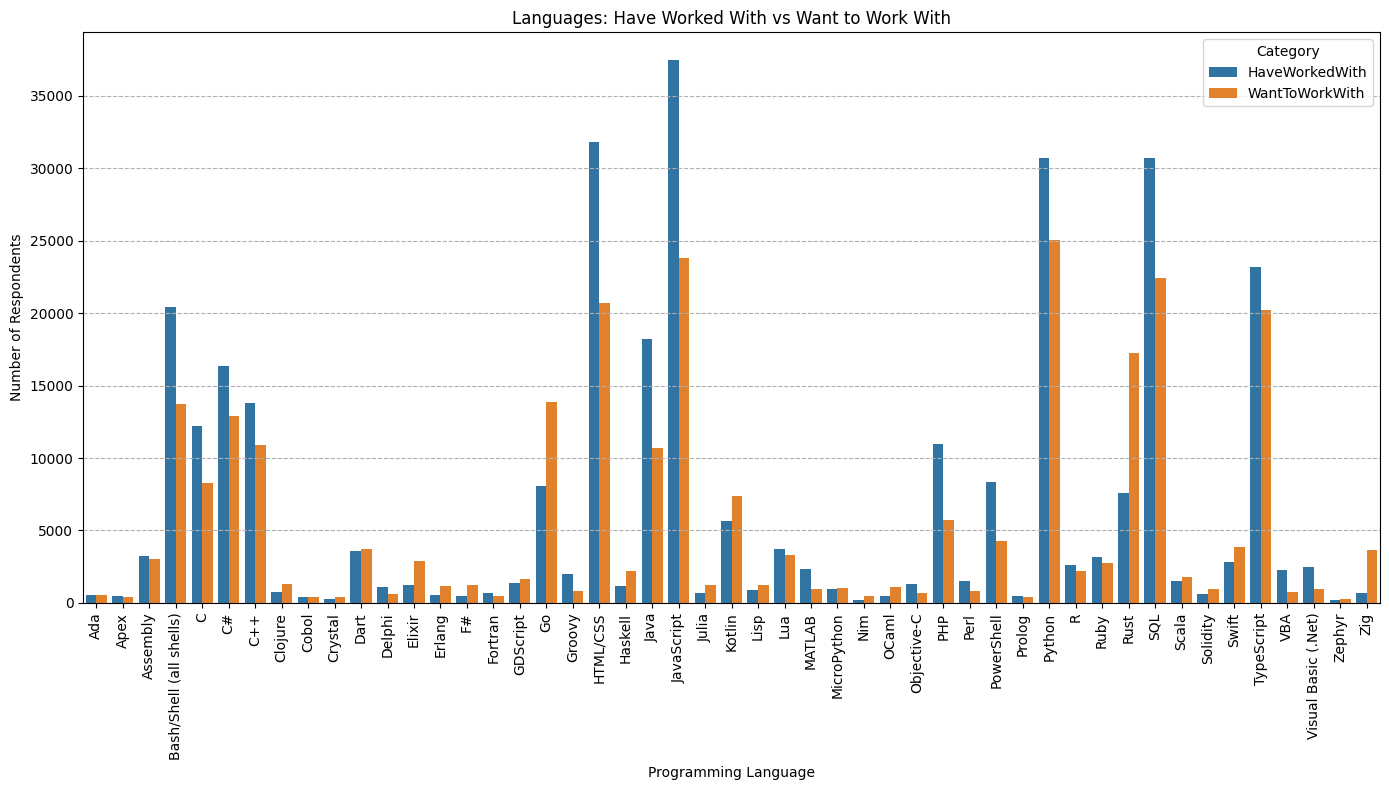
Step 6: Programming Languages Analysis
-
Compare the frequency of programming languages in
LanguageHaveWorkedWithandLanguageWantToWorkWith. -
Visualize the overlap or differences using a Venn diagram or a grouped bar chart.
## Write your code here
for col in ['LanguageHaveWorkedWith', 'LanguageWantToWorkWith']:
    cat = set()
    lang = df_m[col].dropna().unique()
    for el in lang:
        if ';' in el:
            cat = cat | set(el.split(';'))
        else:
            cat.add(el)
    cat = sorted(cat)
    print(col, cat, len(cat))  # Columns that should be added to the dataframe
LanguageHaveWorkedWith ['Ada', 'Apex', 'Assembly', 'Bash/Shell (all shells)', 'C', 'C#', 'C++', 'Clojure', 'Cobol', 'Crystal', 'Dart', 'Delphi', 'Elixir', 'Erlang', 'F#', 'Fortran', 'GDScript', 'Go', 'Groovy', 'HTML/CSS', 'Haskell', 'Java', 'JavaScript', 'Julia', 'Kotlin', 'Lisp', 'Lua', 'MATLAB', 'MicroPython', 'Nim', 'OCaml', 'Objective-C', 'PHP', 'Perl', 'PowerShell', 'Prolog', 'Python', 'R', 'Ruby', 'Rust', 'SQL', 'Scala', 'Solidity', 'Swift', 'TypeScript', 'VBA', 'Visual Basic (.Net)', 'Zephyr', 'Zig'] 49
LanguageWantToWorkWith ['Ada', 'Apex', 'Assembly', 'Bash/Shell (all shells)', 'C', 'C#', 'C++', 'Clojure', 'Cobol', 'Crystal', 'Dart', 'Delphi', 'Elixir', 'Erlang', 'F#', 'Fortran', 'GDScript', 'Go', 'Groovy', 'HTML/CSS', 'Haskell', 'Java', 'JavaScript', 'Julia', 'Kotlin', 'Lisp', 'Lua', 'MATLAB', 'MicroPython', 'Nim', 'OCaml', 'Objective-C', 'PHP', 'Perl', 'PowerShell', 'Prolog', 'Python', 'R', 'Ruby', 'Rust', 'SQL', 'Scala', 'Solidity', 'Swift', 'TypeScript', 'VBA', 'Visual Basic (.Net)', 'Zephyr', 'Zig'] 49
plaWorked = df_m[['LanguageHaveWorkedWith']].dropna()
dummiesWorked = plaWorked['LanguageHaveWorkedWith'].str.get_dummies(sep=';')
plaWorked = dummiesWorked.agg('sum').T

plaWant = df_m[['LanguageWantToWorkWith']].dropna()
dummiesWant = plaWant['LanguageWantToWorkWith'].str.get_dummies(sep=';')
plaWant = dummiesWant.agg('sum').T

pla = pd.concat([plaWorked, plaWant], axis=1)
pla.columns = ['HaveWorkedWith', 'WantToWorkWith']
# Sort languages by HaveWorkedWith (optional but usually helpful)
pla_plot = (pla.reset_index().rename(columns={'index': 'Language'})
    .melt(id_vars='Language',
          var_name='Category',
          value_name='Count'))

plt.figure(figsize=(14, 8))
sns.barplot(
    data=pla_plot,
    x='Language',
    y='Count',
    hue='Category')

plt.xticks(rotation=90)
plt.xlabel("Programming Language")
plt.ylabel("Number of Respondents")
plt.grid(True, axis='y', linestyle='dashed')
plt.title("Languages: Have Worked With vs Want to Work With")
plt.tight_layout()
plt.show()
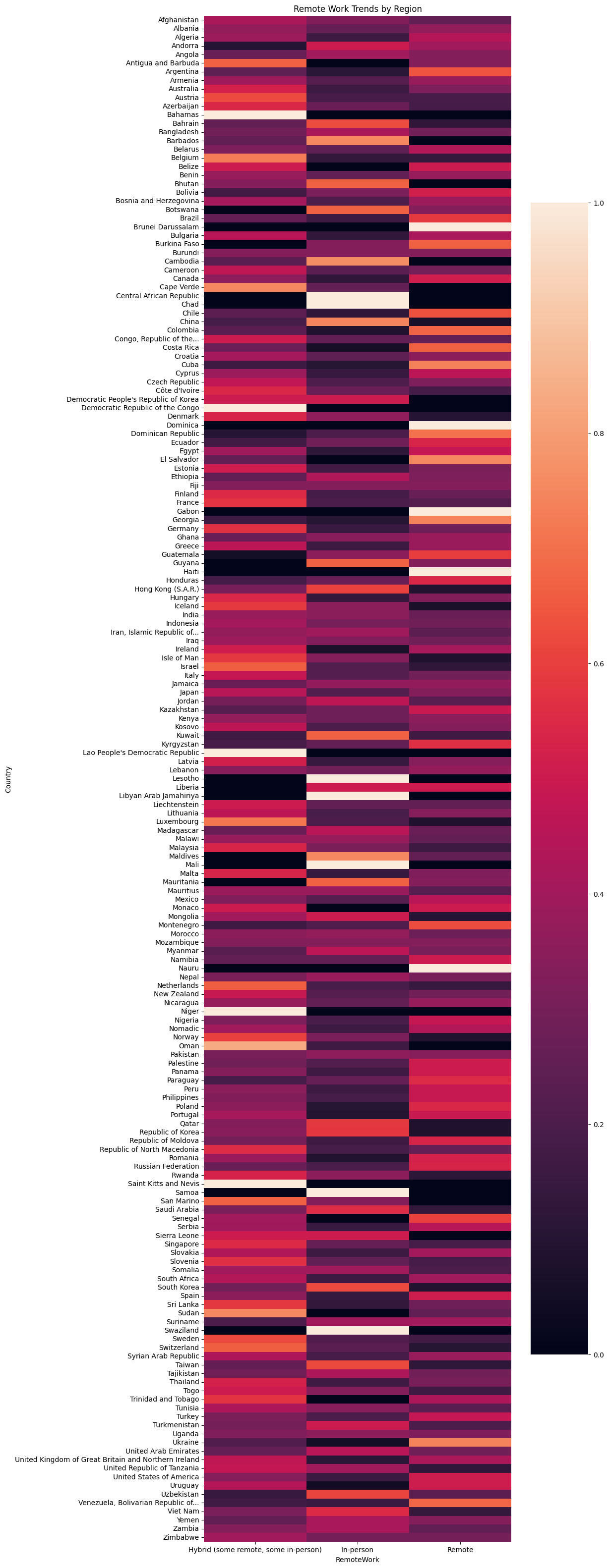
Step 7: Analyze Remote Work Trends
- Visualize the distribution of RemoteWork by region using a grouped bar chart or heatmap.
## Write your code here
rwt = df_m[['Country', 'RemoteWork']].dropna()
rwt_tab = pd.crosstab(rwt.Country, rwt.RemoteWork)
print(rwt_tab.head())
RemoteWork   Hybrid (some remote, some in-person)  In-person  Remote
Country
Afghanistan                                    17         13      10
Albania                                        14         10      14
Algeria                                        19          8      22
Andorra                                         1          5       4
Angola                                          4          6       5
rwt_tabfr = rwt_tab.div(rwt_tab.sum(axis=1), axis=0) # row‑wise normalization

plt.figure(figsize=(10, 40))
sns.heatmap(rwt_tabfr)
plt.title("Remote Work Trends by Region")
plt.show()
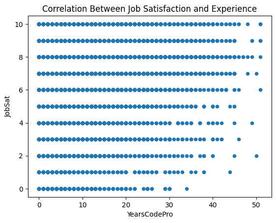
Step 8: Correlation between Job Satisfaction and Experience
-
Analyze the correlation between overall job satisfaction (
JobSat) andYearsCodePro. -
Calculate the Pearson or Spearman correlation coefficient.
## Write your code here
cjsycp = df_m[['JobSat', 'YearsCodePro']].dropna()
cjsycp = cjsycp.replace({'Less than 1 year': 0, 'More than 50 years': 51}).astype(int)

cjsycp.plot(kind='scatter', x='YearsCodePro', y='JobSat')
plt.title('Correlation Between Job Satisfaction and Experience')
plt.ylabel('JobSat')
plt.xlabel('YearsCodePro')
plt.show()
!pip install scipy
from scipy import stats
Collecting scipy
Downloading scipy-1.17.0-cp312-cp312-manylinux_2_27_x86_64.manylinux_2_28_x86_64.whl.metadata (62 kB)
Requirement already satisfied: numpy<2.7,>=1.26.4 in /opt/conda/lib/python3.12/site-packages (from scipy) (2.4.1)
Downloading scipy-1.17.0-cp312-cp312-manylinux_2_27_x86_64.manylinux_2_28_x86_64.whl (35.0 MB)
[2K [90m━━━━━━━━━━━━━━━━━━━━━━━━━━━━━━━━━━━━━━━━[0m [32m35.0/35.0 MB[0m [31m151.1 MB/s[0m eta [36m0:00:00[0m00:01[0m
Installing collected packages: scipy
Successfully installed scipy-1.17.0
pearson_coef, p_valuep = stats.pearsonr(cjsycp['YearsCodePro'], cjsycp['JobSat'])
print("The Pearson Correlation Coefficient is", round(pearson_coef, 4), " with a P-value of P =", round(p_valuep, 4))

spearman_coef, p_values = stats.spearmanr(cjsycp['YearsCodePro'], cjsycp['JobSat'])
print("The Spearman Correlation Coefficient is", round(spearman_coef, 4), " with a P-value of P =", round(p_values, 4))
The Pearson Correlation Coefficient is 0.1042  with a P-value of P = 0.0
The Spearman Correlation Coefficient is 0.1192  with a P-value of P = 0.0
# Values of job satisfaction (JobSat) and Experience (YearsCodePro) show almost no linear or monotonic
# correlation. The correlation values between these two variables are statistically significant.
# The two variables most likely do not affect each other.
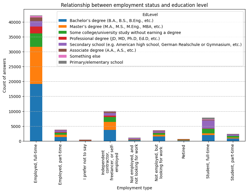
Step 9: Cross-tabulation Analysis (Employment vs. Education Level)
-
Analyze the relationship between employment status (
Employment) and education level (EdLevel). -
Instruction: Create a cross-tabulation using
pd.crosstab()and visualize it with a stacked bar plot if possible.
## Write your code here
emped = df_m[['EdLevel', 'Employment']].dropna()
dummies = emped['Employment'].str.get_dummies(sep=';').astype(bool)
emped = pd.concat([emped, dummies], axis=1).drop(['Employment'], axis=1)
emped_tab = pd.DataFrame()
for col in dummies.columns:
    emped_tab[col] = emped[emped[col]].EdLevel.value_counts()
emped_tab = emped_tab.T.astype(int)
print(emped_tab.head())
EdLevel                                             Bachelor’s degree (B.A., B.S., B.Eng., etc.)  \
Employed, full-time                                                                        19136
Employed, part-time                                                                         1344
I prefer not to say                                                                           96
Independent contractor, freelancer, or self-emp...                                          3711
Not employed, and not looking for work                                                       226

EdLevel                                             Master’s degree (M.A., M.S., M.Eng., MBA, etc.)  \
Employed, full-time                                                                           12489
Employed, part-time                                                                             753
I prefer not to say                                                                              53
Independent contractor, freelancer, or self-emp...                                             2679
Not employed, and not looking for work                                                          110

EdLevel                                             Some college/university study without earning a degree  \
Employed, full-time                                                                              4494
Employed, part-time                                                                               669
I prefer not to say                                                                                51
Independent contractor, freelancer, or self-emp...                                               1634
Not employed, and not looking for work                                                            174

EdLevel                                             Professional degree (JD, MD, Ph.D, Ed.D, etc.)  \
Employed, full-time                                                                           2312
Employed, part-time                                                                            149
I prefer not to say                                                                             29
Independent contractor, freelancer, or self-emp...                                             485
Not employed, and not looking for work                                                          23

EdLevel                                             Secondary school (e.g. American high school, German Realschule or Gymnasium, etc.)  \
Employed, full-time                                                                              1860
Employed, part-time                                                                               623
I prefer not to say                                                                                92
Independent contractor, freelancer, or self-emp...                                                902
Not employed, and not looking for work                                                            338

EdLevel                                             Associate degree (A.A., A.S., etc.)  \
Employed, full-time                                                                1260
Employed, part-time                                                                 137
I prefer not to say                                                                   9
Independent contractor, freelancer, or self-emp...                                  323
Not employed, and not looking for work                                               22

EdLevel                                             Something else  \
Employed, full-time                                            448
Employed, part-time                                             69
I prefer not to say                                             83
Independent contractor, freelancer, or self-emp...             145
Not employed, and not looking for work                          45

EdLevel                                             Primary/elementary school
Employed, full-time                                                       201
Employed, part-time                                                        79
I prefer not to say                                                        51
Independent contractor, freelancer, or self-emp...                        159
Not employed, and not looking for work                                    155
ax = emped_tab.plot(kind='bar', figsize=(10, 6), stacked=True)

xlabels = [textwrap.fill(label.get_text(), width=20) for label in ax.get_xticklabels()]
ax.set(xlabel='Employment type', ylabel='Count of answers')
ax.set_xticklabels(xlabels)
plt.title('Relationship between employment status and education level')
plt.grid(True, axis='y', linestyle='dashed')

plt.show()
Step 10: Export Cleaned Data
- Save the cleaned dataset to a new CSV file for further use or sharing.
## Write your code here
df_m.to_csv("Lab13out.csv", index=False)
Summary:
In this lab, you practiced key skills in exploratory data analysis, including:
-
Examining the structure and content of the Stack Overflow survey dataset to understand its variables and data types.
-
Identifying and addressing missing data to ensure the dataset's quality and completeness.
-
Summarizing and visualizing key variables such as job satisfaction, programming languages, and remote work trends.
-
Analyzing relationships in the data using techniques like:
-
Comparing programming languages respondents have worked with versus those they want to work with.
-
Exploring remote work preferences by region.
-
-
Investigating correlations between professional coding experience and job satisfaction.
-
Performing cross-tabulations to analyze relationships between employment status and education levels.
Authors:
Ayushi Jain
Other Contributors:
Rav Ahuja Lakshmi Holla Malika
Copyright © IBM Corporation. All rights reserved.