Finding Outliers

Estimated time needed: 30 minutes

In this lab, you will work with a cleaned dataset to perform exploratory data analysis or EDA. You will explore the distribution of key variables and focus on identifying outliers in this lab.

Objectives

In this lab, you will perform the following:

Analyze the distribution of key variables in the dataset.
Identify and remove outliers using statistical methods.
Perform relevant statistical and correlation analysis.

Install and import the required libraries

!pip install pandas
!pip install matplotlib
!pip install seaborn
!pip install scipy

import pandas as pd
import matplotlib.pyplot as plt
import seaborn as sns
from scipy import stats
import textwrap

Requirement already satisfied: pandas in /opt/conda/lib/python3.12/site-packages (3.0.0)
Requirement already satisfied: numpy>=1.26.0 in /opt/conda/lib/python3.12/site-packages (from pandas) (2.4.2)
Requirement already satisfied: python-dateutil>=2.8.2 in /opt/conda/lib/python3.12/site-packages (from pandas) (2.9.0.post0)
Requirement already satisfied: six>=1.5 in /opt/conda/lib/python3.12/site-packages (from python-dateutil>=2.8.2->pandas) (1.17.0)
Requirement already satisfied: matplotlib in /opt/conda/lib/python3.12/site-packages (3.10.8)
Requirement already satisfied: contourpy>=1.0.1 in /opt/conda/lib/python3.12/site-packages (from matplotlib) (1.3.3)
Requirement already satisfied: cycler>=0.10 in /opt/conda/lib/python3.12/site-packages (from matplotlib) (0.12.1)
Requirement already satisfied: fonttools>=4.22.0 in /opt/conda/lib/python3.12/site-packages (from matplotlib) (4.61.1)
Requirement already satisfied: kiwisolver>=1.3.1 in /opt/conda/lib/python3.12/site-packages (from matplotlib) (1.4.9)
Requirement already satisfied: numpy>=1.23 in /opt/conda/lib/python3.12/site-packages (from matplotlib) (2.4.2)
Requirement already satisfied: packaging>=20.0 in /opt/conda/lib/python3.12/site-packages (from matplotlib) (24.2)
Requirement already satisfied: pillow>=8 in /opt/conda/lib/python3.12/site-packages (from matplotlib) (12.1.0)
Requirement already satisfied: pyparsing>=3 in /opt/conda/lib/python3.12/site-packages (from matplotlib) (3.3.2)
Requirement already satisfied: python-dateutil>=2.7 in /opt/conda/lib/python3.12/site-packages (from matplotlib) (2.9.0.post0)
Requirement already satisfied: six>=1.5 in /opt/conda/lib/python3.12/site-packages (from python-dateutil>=2.7->matplotlib) (1.17.0)
Requirement already satisfied: seaborn in /opt/conda/lib/python3.12/site-packages (0.13.2)
Requirement already satisfied: numpy!=1.24.0,>=1.20 in /opt/conda/lib/python3.12/site-packages (from seaborn) (2.4.2)
Requirement already satisfied: pandas>=1.2 in /opt/conda/lib/python3.12/site-packages (from seaborn) (3.0.0)
Requirement already satisfied: matplotlib!=3.6.1,>=3.4 in /opt/conda/lib/python3.12/site-packages (from seaborn) (3.10.8)
Requirement already satisfied: contourpy>=1.0.1 in /opt/conda/lib/python3.12/site-packages (from matplotlib!=3.6.1,>=3.4->seaborn) (1.3.3)
Requirement already satisfied: cycler>=0.10 in /opt/conda/lib/python3.12/site-packages (from matplotlib!=3.6.1,>=3.4->seaborn) (0.12.1)
Requirement already satisfied: fonttools>=4.22.0 in /opt/conda/lib/python3.12/site-packages (from matplotlib!=3.6.1,>=3.4->seaborn) (4.61.1)
Requirement already satisfied: kiwisolver>=1.3.1 in /opt/conda/lib/python3.12/site-packages (from matplotlib!=3.6.1,>=3.4->seaborn) (1.4.9)
Requirement already satisfied: packaging>=20.0 in /opt/conda/lib/python3.12/site-packages (from matplotlib!=3.6.1,>=3.4->seaborn) (24.2)
Requirement already satisfied: pillow>=8 in /opt/conda/lib/python3.12/site-packages (from matplotlib!=3.6.1,>=3.4->seaborn) (12.1.0)
Requirement already satisfied: pyparsing>=3 in /opt/conda/lib/python3.12/site-packages (from matplotlib!=3.6.1,>=3.4->seaborn) (3.3.2)
Requirement already satisfied: python-dateutil>=2.7 in /opt/conda/lib/python3.12/site-packages (from matplotlib!=3.6.1,>=3.4->seaborn) (2.9.0.post0)
Requirement already satisfied: six>=1.5 in /opt/conda/lib/python3.12/site-packages (from python-dateutil>=2.7->matplotlib!=3.6.1,>=3.4->seaborn) (1.17.0)
Requirement already satisfied: scipy in /opt/conda/lib/python3.12/site-packages (1.17.0)
Requirement already satisfied: numpy<2.7,>=1.26.4 in /opt/conda/lib/python3.12/site-packages (from scipy) (2.4.2)

Step 1: Load and Explore the Dataset

Load the dataset into a DataFrame and examine the structure of the data.

file_url = "https://cf-courses-data.s3.us.cloud-object-storage.appdomain.cloud/n01PQ9pSmiRX6520flujwQ/survey-data.csv"

#Create the dataframe
df = pd.read_csv(file_url)

#Display the top 10 records
print(df.head())
print('Initial dataframe:', df.shape)

   ResponseId                      MainBranch                 Age  \
0           1  I am a developer by profession  Under 18 years old   
1           2  I am a developer by profession     35-44 years old   
2           3  I am a developer by profession     45-54 years old   
3           4           I am learning to code     18-24 years old   
4           5  I am a developer by profession     18-24 years old   

            Employment RemoteWork   Check  \
0  Employed, full-time     Remote  Apples   
1  Employed, full-time     Remote  Apples   
2  Employed, full-time     Remote  Apples   
3   Student, full-time        NaN  Apples   
4   Student, full-time        NaN  Apples   

                                    CodingActivities  \
0                                              Hobby   
1  Hobby;Contribute to open-source projects;Other...   
2  Hobby;Contribute to open-source projects;Other...   
3                                                NaN   
4                                                NaN   

                                             EdLevel  \
0                          Primary/elementary school   
1       Bachelor’s degree (B.A., B.S., B.Eng., etc.)   
2    Master’s degree (M.A., M.S., M.Eng., MBA, etc.)   
3  Some college/university study without earning ...   
4  Secondary school (e.g. American high school, G...   

                                           LearnCode  \
0                             Books / Physical media   
1  Books / Physical media;Colleague;On the job tr...   
2  Books / Physical media;Colleague;On the job tr...   
3  Other online resources (e.g., videos, blogs, f...   
4  Other online resources (e.g., videos, blogs, f...   

                                     LearnCodeOnline  ... JobSatPoints_6  \
0                                                NaN  ...            NaN   
1  Technical documentation;Blogs;Books;Written Tu...  ...            0.0   
2  Technical documentation;Blogs;Books;Written Tu...  ...            NaN   
3  Stack Overflow;How-to videos;Interactive tutorial  ...            NaN   
4  Technical documentation;Blogs;Written Tutorial...  ...            NaN   

  JobSatPoints_7 JobSatPoints_8 JobSatPoints_9 JobSatPoints_10  \
0            NaN            NaN            NaN             NaN   
1            0.0            0.0            0.0             0.0   
2            NaN            NaN            NaN             NaN   
3            NaN            NaN            NaN             NaN   
4            NaN            NaN            NaN             NaN   

  JobSatPoints_11           SurveyLength SurveyEase ConvertedCompYearly JobSat  
0             NaN                    NaN        NaN                 NaN    NaN  
1             0.0                    NaN        NaN                 NaN    NaN  
2             NaN  Appropriate in length       Easy                 NaN    NaN  
3             NaN               Too long       Easy                 NaN    NaN  
4             NaN              Too short       Easy                 NaN    NaN  

[5 rows x 114 columns]
Initial dataframe: (65437, 114)

Step 2: Plot the Distribution of Industry

Explore how respondents are distributed across different industries.

Plot a bar chart to visualize the distribution of respondents by industry.
Highlight any notable trends.

##Write your code here
pdi = df.dropna(subset=['Industry'])

plt.figure(figsize=(14, 8))
order = pdi['Industry'].value_counts().index  # the bars in descending order
ax = sns.countplot(data=pdi, x='Industry', order=order)
labels = [textwrap.fill(label.get_text(), width=20) for label in ax.get_xticklabels()]
ax.set(xticklabels=labels)
plt.xticks(rotation=90)
plt.xlabel("Type of Industry")
plt.ylabel("Number of Respondents")
plt.grid(True, axis='y', linestyle='dashed')
plt.title("Distribution of respondents by industry")
plt.tight_layout()
plt.show()

/tmp/ipykernel_300/1847729545.py:8: UserWarning: set_ticklabels() should only be used with a fixed number of ticks, i.e. after set_ticks() or using a FixedLocator.
  ax.set(xticklabels=labels)

png

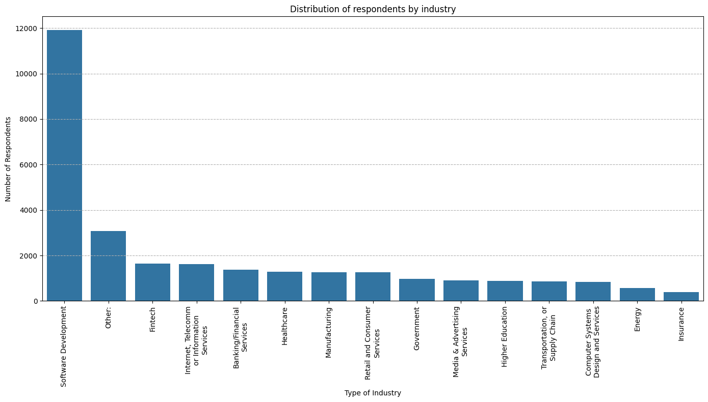
# Most respondents work in Software development.

Step 3: Identify High Compensation Outliers

Identify respondents with extremely high yearly compensation.

Calculate basic statistics (mean, median, and standard deviation) for ConvertedCompYearly.
Identify compensation values exceeding a defined threshold (e.g., 3 standard deviations above the mean).

##Write your code here
ihco = df.dropna(subset=['ConvertedCompYearly'])
print(ihco.ConvertedCompYearly.describe().astype(int))

count       23435
mean        86155
std        186756
min             1
25%         32712
50%         65000
75%        107971
max      16256603
Name: ConvertedCompYearly, dtype: int64

stdev = ihco.ConvertedCompYearly.std()
average = ihco.ConvertedCompYearly.mean()
outliers1 = ihco[ihco['ConvertedCompYearly'] > average + 3 * stdev]['ConvertedCompYearly'].sort_values(ascending=False).unique()
print(outliers1)

[16256603. 13818022.  9000000.  6340564.  4936778.  3367716.  2584118.
  2237846.  2153432.  2048046.  2014062.  2000000.  1900000.  1750749.
  1750000.  1728025.  1562898.  1550391.  1500000.  1332930.  1302817.
  1300000.  1295242.  1288874.  1273879.  1250348.  1200000.  1188001.
  1184707.  1140481.  1074062.  1052581.  1031099.  1000000.   980887.
   950000.   945000.   912953.   900000.   875000.   859250.   850000.
   810000.   803285.   800000.   798000.   764327.   750000.   740517.
   720000.   713372.   712801.   700000.   675000.   670000.   660660.
   650000.]

Step 4: Detect Outliers in Compensation

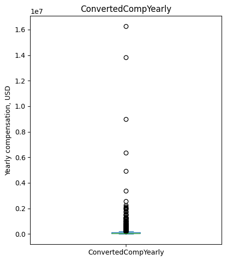
Identify outliers in the ConvertedCompYearly column using the IQR method.

Calculate the Interquartile Range (IQR).
Determine the upper and lower bounds for outliers.
Count and visualize outliers using a box plot.

##Write your code here
doc = ihco.ConvertedCompYearly
q1, q3 = doc.quantile(.25), doc.quantile(.75)
iqr = q3 - q1
outliers2 = doc[(doc > q3 + 1.5 * iqr) | (doc < q1 - 1.5 * iqr)].sort_values(ascending=False)
print('Number of outliers in ConvertedCompYearly:', outliers2.count())

Number of outliers in ConvertedCompYearly: 978

doc.plot(kind='box', figsize=(5, 6))

plt.title('ConvertedCompYearly')
plt.ylabel('Yearly compensation, USD')

plt.show()

png

Step 5: Remove Outliers and Create a New DataFrame

Remove outliers from the dataset.

Create a new DataFrame excluding rows with outliers in ConvertedCompYearly.
Validate the size of the new DataFrame.

##Write your code here
df_o = df[~df['ConvertedCompYearly'].isin(outliers2)]
df_o['ConvertedCompYearly'].describe()

count     22457.000000
mean      71347.201897
std       51271.396445
min           1.000000
25%       32000.000000
50%       63694.000000
75%      101281.000000
max      220207.000000
Name: ConvertedCompYearly, dtype: float64

Step 6: Correlation Analysis

Analyze the correlation between Age (transformed) and other numerical columns.

Map the Age column to approximate numeric values.
Compute correlations between Age and other numeric variables.
Visualize the correlation matrix.

Age = df.Age
Age = Age.map({'Under 18 years old': 17, '18-24 years old': 21, 'Prefer not to say': float('nan'), 
        '25-34 years old': 30, '35-44 years old': 40, '45-54 years old': 50,
        '55-64 years old': 60, '65 years or older': 66})
Age.unique()

array([17., 40., 50., 21., 30., 60., nan, 66.])

df_corr = df.copy()
df_corr.Age = Age
df_corr.corr(numeric_only=True)

	ResponseId	Age	CompTotal	WorkExp	JobSatPoints_1	JobSatPoints_4	JobSatPoints_5	JobSatPoints_6	JobSatPoints_7	JobSatPoints_8	JobSatPoints_9	JobSatPoints_10	JobSatPoints_11	ConvertedCompYearly	JobSat
ResponseId	1.000000	-0.038339	-0.000000	0.011955	-0.002406	-0.015738	-0.014197	-0.001908	0.001843	-0.002968	0.001991	-0.005365	-0.005865	-0.008363	0.002425
Age	-0.038339	1.000000	-0.002709	0.848165	-0.027672	-0.076214	-0.101811	-0.050353	-0.083718	-0.046519	-0.082170	-0.114871	-0.107356	0.122590	0.069514
CompTotal	-0.000000	-0.002709	0.000000	0.028766	-0.004891	-0.002719	-0.003033	-0.006311	-0.005893	-0.004585	-0.004494	-0.003198	-0.003045	0.080457	-0.015770
WorkExp	0.011955	0.848165	0.028766	1.000000	-0.026490	-0.067241	-0.104525	-0.065352	-0.101461	-0.046958	-0.088090	-0.113707	-0.108279	0.154114	0.097322
JobSatPoints_1	-0.002406	-0.027672	-0.004891	-0.026490	1.000000	0.445710	0.633765	0.618618	0.603157	0.627385	0.597527	0.585087	0.607792	0.020306	0.094068
JobSatPoints_4	-0.015738	-0.076214	-0.002719	-0.067241	0.445710	1.000000	0.526254	0.449400	0.459253	0.438763	0.472516	0.499387	0.528395	0.018197	0.029677
JobSatPoints_5	-0.014197	-0.101811	-0.003033	-0.104525	0.633765	0.526254	1.000000	0.613933	0.607949	0.630353	0.619644	0.643538	0.690993	-0.023281	0.049224
JobSatPoints_6	-0.001908	-0.050353	-0.006311	-0.065352	0.618618	0.449400	0.613933	1.000000	0.692166	0.645094	0.632211	0.592528	0.604585	-0.008518	0.051341
JobSatPoints_7	0.001843	-0.083718	-0.005893	-0.101461	0.603157	0.459253	0.607949	0.692166	1.000000	0.698240	0.659558	0.642905	0.618444	-0.036431	0.038339
JobSatPoints_8	-0.002968	-0.046519	-0.004585	-0.046958	0.627385	0.438763	0.630353	0.645094	0.698240	1.000000	0.655668	0.617320	0.625185	-0.011080	0.058258
JobSatPoints_9	0.001991	-0.082170	-0.004494	-0.088090	0.597527	0.472516	0.619644	0.632211	0.659558	0.655668	1.000000	0.663628	0.650676	-0.015867	0.039173
JobSatPoints_10	-0.005365	-0.114871	-0.003198	-0.113707	0.585087	0.499387	0.643538	0.592528	0.642905	0.617320	0.663628	1.000000	0.737598	-0.022228	0.045063
JobSatPoints_11	-0.005865	-0.107356	-0.003045	-0.108279	0.607792	0.528395	0.690993	0.604585	0.618444	0.625185	0.650676	0.737598	1.000000	-0.010038	0.045093
ConvertedCompYearly	-0.008363	0.122590	0.080457	0.154114	0.020306	0.018197	-0.023281	-0.008518	-0.036431	-0.011080	-0.015867	-0.022228	-0.010038	1.000000	0.048428
JobSat	0.002425	0.069514	-0.015770	0.097322	0.094068	0.029677	0.049224	0.051341	0.038339	0.058258	0.039173	0.045063	0.045093	0.048428	1.000000

Summary

In this lab, you developed essential skills in Exploratory Data Analysis (EDA) with a focus on outlier detection and removal. Specifically, you:

Loaded and explored the dataset to understand its structure.
Analyzed the distribution of respondents across industries.
Identified and removed high compensation outliers using statistical thresholds and the Interquartile Range (IQR) method.
Performed correlation analysis, including transforming the Age column into numeric values for better analysis.