
Pie Charts
Estimated time needed: 30 minutes
-
In this lab, you will focus on visualizing data.
-
The provided dataset will be loaded into pandas for analysis.
-
Various pie charts will be created to:
-
Analyze developer preferences.
-
Identify technology usage trends.
-
-
The lab aims to provide insights into key variables using visual representations.
Objectives
In this lab you will perform the following:
-
Visualize the distribution of data.
-
Visualize the relationship between two features.
-
Visualize composition of data.
-
Visualize comparison of data.
Setup: Downloading and Loading the Data
Install the libraries
!pip install pandas
Collecting pandas
Downloading pandas-3.0.0-cp312-cp312-manylinux_2_24_x86_64.manylinux_2_28_x86_64.whl.metadata (79 kB)
Collecting numpy>=1.26.0 (from pandas)
Downloading numpy-2.4.2-cp312-cp312-manylinux_2_27_x86_64.manylinux_2_28_x86_64.whl.metadata (6.6 kB)
Requirement already satisfied: python-dateutil>=2.8.2 in /opt/conda/lib/python3.12/site-packages (from pandas) (2.9.0.post0)
Requirement already satisfied: six>=1.5 in /opt/conda/lib/python3.12/site-packages (from python-dateutil>=2.8.2->pandas) (1.17.0)
Downloading pandas-3.0.0-cp312-cp312-manylinux_2_24_x86_64.manylinux_2_28_x86_64.whl (10.9 MB)
[2K [90m━━━━━━━━━━━━━━━━━━━━━━━━━━━━━━━━━━━━━━━━[0m [32m10.9/10.9 MB[0m [31m106.0 MB/s[0m eta [36m0:00:00[0m
[?25hDownloading numpy-2.4.2-cp312-cp312-manylinux_2_27_x86_64.manylinux_2_28_x86_64.whl (16.6 MB)
[2K [90m━━━━━━━━━━━━━━━━━━━━━━━━━━━━━━━━━━━━━━━━[0m [32m16.6/16.6 MB[0m [31m191.2 MB/s[0m eta [36m0:00:00[0m
Installing collected packages: numpy, pandas
Successfully installed numpy-2.4.2 pandas-3.0.0
!pip install matplotlib
!pip install seaborn
Collecting matplotlib
Downloading matplotlib-3.10.8-cp312-cp312-manylinux2014_x86_64.manylinux_2_17_x86_64.whl.metadata (52 kB)
Collecting contourpy>=1.0.1 (from matplotlib)
Downloading contourpy-1.3.3-cp312-cp312-manylinux_2_27_x86_64.manylinux_2_28_x86_64.whl.metadata (5.5 kB)
Collecting cycler>=0.10 (from matplotlib)
Downloading cycler-0.12.1-py3-none-any.whl.metadata (3.8 kB)
Collecting fonttools>=4.22.0 (from matplotlib)
Downloading fonttools-4.61.1-cp312-cp312-manylinux1_x86_64.manylinux2014_x86_64.manylinux_2_17_x86_64.manylinux_2_5_x86_64.whl.metadata (114 kB)
Collecting kiwisolver>=1.3.1 (from matplotlib)
Downloading kiwisolver-1.4.9-cp312-cp312-manylinux2014_x86_64.manylinux_2_17_x86_64.whl.metadata (6.3 kB)
Requirement already satisfied: numpy>=1.23 in /opt/conda/lib/python3.12/site-packages (from matplotlib) (2.4.2)
Requirement already satisfied: packaging>=20.0 in /opt/conda/lib/python3.12/site-packages (from matplotlib) (24.2)
Collecting pillow>=8 (from matplotlib)
Downloading pillow-12.1.0-cp312-cp312-manylinux_2_27_x86_64.manylinux_2_28_x86_64.whl.metadata (8.8 kB)
Collecting pyparsing>=3 (from matplotlib)
Downloading pyparsing-3.3.2-py3-none-any.whl.metadata (5.8 kB)
Requirement already satisfied: python-dateutil>=2.7 in /opt/conda/lib/python3.12/site-packages (from matplotlib) (2.9.0.post0)
Requirement already satisfied: six>=1.5 in /opt/conda/lib/python3.12/site-packages (from python-dateutil>=2.7->matplotlib) (1.17.0)
Downloading matplotlib-3.10.8-cp312-cp312-manylinux2014_x86_64.manylinux_2_17_x86_64.whl (8.7 MB)
[2K [90m━━━━━━━━━━━━━━━━━━━━━━━━━━━━━━━━━━━━━━━━[0m [32m8.7/8.7 MB[0m [31m200.6 MB/s[0m eta [36m0:00:00[0m
[?25hDownloading contourpy-1.3.3-cp312-cp312-manylinux_2_27_x86_64.manylinux_2_28_x86_64.whl (362 kB)
Downloading cycler-0.12.1-py3-none-any.whl (8.3 kB)
Downloading fonttools-4.61.1-cp312-cp312-manylinux1_x86_64.manylinux2014_x86_64.manylinux_2_17_x86_64.manylinux_2_5_x86_64.whl (5.0 MB)
[2K [90m━━━━━━━━━━━━━━━━━━━━━━━━━━━━━━━━━━━━━━━━[0m [32m5.0/5.0 MB[0m [31m175.7 MB/s[0m eta [36m0:00:00[0m
[?25hDownloading kiwisolver-1.4.9-cp312-cp312-manylinux2014_x86_64.manylinux_2_17_x86_64.whl (1.5 MB)
[2K [90m━━━━━━━━━━━━━━━━━━━━━━━━━━━━━━━━━━━━━━━━[0m [32m1.5/1.5 MB[0m [31m105.1 MB/s[0m eta [36m0:00:00[0m
[?25hDownloading pillow-12.1.0-cp312-cp312-manylinux_2_27_x86_64.manylinux_2_28_x86_64.whl (7.0 MB)
[2K [90m━━━━━━━━━━━━━━━━━━━━━━━━━━━━━━━━━━━━━━━━[0m [32m7.0/7.0 MB[0m [31m142.3 MB/s[0m eta [36m0:00:00[0m
[?25hDownloading pyparsing-3.3.2-py3-none-any.whl (122 kB)
Installing collected packages: pyparsing, pillow, kiwisolver, fonttools, cycler, contourpy, matplotlib
Successfully installed contourpy-1.3.3 cycler-0.12.1 fonttools-4.61.1 kiwisolver-1.4.9 matplotlib-3.10.8 pillow-12.1.0 pyparsing-3.3.2
Collecting seaborn
Downloading seaborn-0.13.2-py3-none-any.whl.metadata (5.4 kB)
Requirement already satisfied: numpy!=1.24.0,>=1.20 in /opt/conda/lib/python3.12/site-packages (from seaborn) (2.4.2)
Requirement already satisfied: pandas>=1.2 in /opt/conda/lib/python3.12/site-packages (from seaborn) (3.0.0)
Requirement already satisfied: matplotlib!=3.6.1,>=3.4 in /opt/conda/lib/python3.12/site-packages (from seaborn) (3.10.8)
Requirement already satisfied: contourpy>=1.0.1 in /opt/conda/lib/python3.12/site-packages (from matplotlib!=3.6.1,>=3.4->seaborn) (1.3.3)
Requirement already satisfied: cycler>=0.10 in /opt/conda/lib/python3.12/site-packages (from matplotlib!=3.6.1,>=3.4->seaborn) (0.12.1)
Requirement already satisfied: fonttools>=4.22.0 in /opt/conda/lib/python3.12/site-packages (from matplotlib!=3.6.1,>=3.4->seaborn) (4.61.1)
Requirement already satisfied: kiwisolver>=1.3.1 in /opt/conda/lib/python3.12/site-packages (from matplotlib!=3.6.1,>=3.4->seaborn) (1.4.9)
Requirement already satisfied: packaging>=20.0 in /opt/conda/lib/python3.12/site-packages (from matplotlib!=3.6.1,>=3.4->seaborn) (24.2)
Requirement already satisfied: pillow>=8 in /opt/conda/lib/python3.12/site-packages (from matplotlib!=3.6.1,>=3.4->seaborn) (12.1.0)
Requirement already satisfied: pyparsing>=3 in /opt/conda/lib/python3.12/site-packages (from matplotlib!=3.6.1,>=3.4->seaborn) (3.3.2)
Requirement already satisfied: python-dateutil>=2.7 in /opt/conda/lib/python3.12/site-packages (from matplotlib!=3.6.1,>=3.4->seaborn) (2.9.0.post0)
Requirement already satisfied: six>=1.5 in /opt/conda/lib/python3.12/site-packages (from python-dateutil>=2.7->matplotlib!=3.6.1,>=3.4->seaborn) (1.17.0)
Downloading seaborn-0.13.2-py3-none-any.whl (294 kB)
Installing collected packages: seaborn
Successfully installed seaborn-0.13.2
Download and Load the Data
To start, download and load the dataset into a pandas DataFrame.
# Step 1: Download the dataset
!wget -O survey-data.csv https://cf-courses-data.s3.us.cloud-object-storage.appdomain.cloud/n01PQ9pSmiRX6520flujwQ/survey-data.csv

# Step 2: Import necessary libraries and load the dataset
import pandas as pd
import matplotlib.pyplot as plt
import seaborn as sns
import textwrap
import numpy as np

# Load the data
df = pd.read_csv("survey-data.csv")

# Display the first few rows to understand the structure of the data
print(df.head())
print('Initial dataframe:', df.shape)
--2026-02-10 08:17:08--  https://cf-courses-data.s3.us.cloud-object-storage.appdomain.cloud/n01PQ9pSmiRX6520flujwQ/survey-data.csv
Resolving cf-courses-data.s3.us.cloud-object-storage.appdomain.cloud (cf-courses-data.s3.us.cloud-object-storage.appdomain.cloud)... 169.63.118.104
Connecting to cf-courses-data.s3.us.cloud-object-storage.appdomain.cloud (cf-courses-data.s3.us.cloud-object-storage.appdomain.cloud)|169.63.118.104|:443... connected.
200 OKequest sent, awaiting response...
Length: 159525875 (152M) [text/csv]
Saving to: ‘survey-data.csv’

survey-data.csv     100%[===================>] 152.13M  70.7MB/s    in 2.2s

2026-02-10 08:17:10 (70.7 MB/s) - ‘survey-data.csv’ saved [159525875/159525875]

   ResponseId                      MainBranch                 Age  \
0           1  I am a developer by profession  Under 18 years old
1           2  I am a developer by profession     35-44 years old
2           3  I am a developer by profession     45-54 years old
3           4           I am learning to code     18-24 years old
4           5  I am a developer by profession     18-24 years old

            Employment RemoteWork   Check  \
0  Employed, full-time     Remote  Apples
1  Employed, full-time     Remote  Apples
2  Employed, full-time     Remote  Apples
3   Student, full-time        NaN  Apples
4   Student, full-time        NaN  Apples

                                    CodingActivities  \
0                                              Hobby
1  Hobby;Contribute to open-source projects;Other...
2  Hobby;Contribute to open-source projects;Other...
3                                                NaN
4                                                NaN

                                             EdLevel  \
0                          Primary/elementary school
1       Bachelor’s degree (B.A., B.S., B.Eng., etc.)
2    Master’s degree (M.A., M.S., M.Eng., MBA, etc.)
3  Some college/university study without earning ...
4  Secondary school (e.g. American high school, G...

                                           LearnCode  \
0                             Books / Physical media
1  Books / Physical media;Colleague;On the job tr...
2  Books / Physical media;Colleague;On the job tr...
3  Other online resources (e.g., videos, blogs, f...
4  Other online resources (e.g., videos, blogs, f...

                                     LearnCodeOnline  ... JobSatPoints_6  \
0                                                NaN  ...            NaN
1  Technical documentation;Blogs;Books;Written Tu...  ...            0.0
2  Technical documentation;Blogs;Books;Written Tu...  ...            NaN
3  Stack Overflow;How-to videos;Interactive tutorial  ...            NaN
4  Technical documentation;Blogs;Written Tutorial...  ...            NaN

  JobSatPoints_7 JobSatPoints_8 JobSatPoints_9 JobSatPoints_10  \
0            NaN            NaN            NaN             NaN
1            0.0            0.0            0.0             0.0
2            NaN            NaN            NaN             NaN
3            NaN            NaN            NaN             NaN
4            NaN            NaN            NaN             NaN

  JobSatPoints_11           SurveyLength SurveyEase ConvertedCompYearly JobSat
0             NaN                    NaN        NaN                 NaN    NaN
1             0.0                    NaN        NaN                 NaN    NaN
2             NaN  Appropriate in length       Easy                 NaN    NaN
3             NaN               Too long       Easy                 NaN    NaN
4             NaN              Too short       Easy                 NaN    NaN

[5 rows x 114 columns]
Initial dataframe: (65437, 114)
Task 1: Visualizing Data Composition with Pie Charts
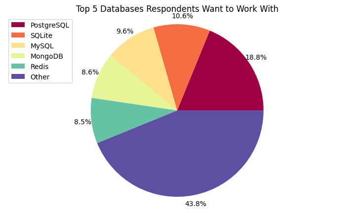
1.1 Create a Pie Chart of the Top 5 Databases Respondents Want to Work With
In the survey data, the DatabaseWantToWorkWith column lists the databases that respondents wish to work with. Let’s visualize the top 5 most-desired databases in a pie chart.
##Write your code here
dummies = df['DatabaseWantToWorkWith'].str.get_dummies(sep=';')
# Count total occurrences and sort
counts = dummies.sum().sort_values(ascending=False)
# Build Top 5 + Other
top5 = counts.iloc[:5]
other = counts.iloc[5:].sum()
databp = pd.concat([top5, pd.Series({'Other': other})])

databp.plot(kind='pie',
              figsize=(9, 5),
              autopct='%1.1f%%', # add in percentages
              labels=None,
              startangle=0,
              pctdistance=1.10,  # the ratio between the center of each pie slice and the start of the text
              shadow=False,
              colormap='Spectral')

plt.title('Top 5 Databases Respondents Want to Work With')
plt.axis('equal') # Sets the pie chart to look like a circle
plt.legend(labels=databp.index, loc='upper left')

plt.show()
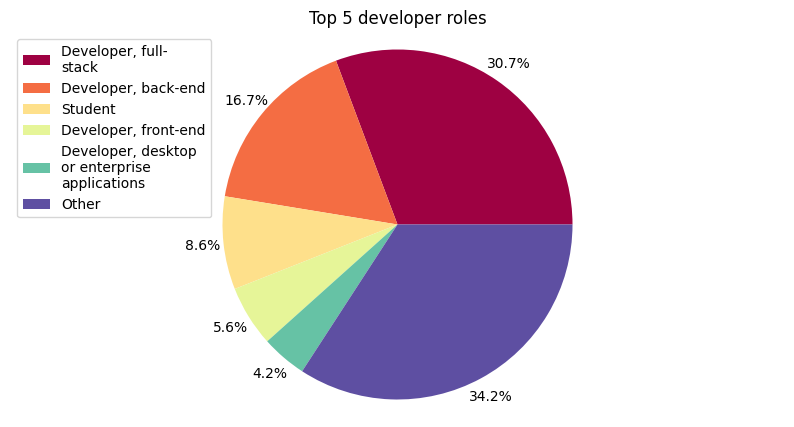
The DevType column lists the developer types for respondents. We’ll examine the distribution by showing the top 5 developer roles in a pie chart.
##Write your code here
dev = df.DevType.value_counts()
top5 = dev.iloc[:5]
other = dev.iloc[5:].sum()
devp = pd.concat([top5, pd.Series({'Other': other})])
devp.plot(kind='pie',
              figsize=(10, 5),
              autopct='%1.1f%%', # add in percentages
              labels=None,
              startangle=0,
              pctdistance=1.12,  # the ratio between the center of each pie slice and the start of the text
              shadow=False,
              colormap='Spectral')

plt.title('Top 5 developer roles')
plt.axis('equal') # Sets the pie chart to look like a circle
wrapped_labels = ['\n'.join(textwrap.wrap(label, 20)) for label in devp.index]
plt.legend(labels=wrapped_labels, loc='upper left')

plt.show()
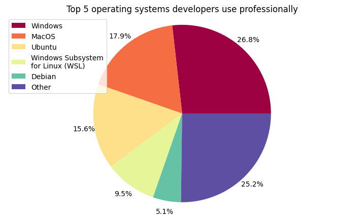
1.3 Create a pie chart for the operating systems used by respondents for professional use
The OpSysProfessional use column shows the operating systems developers use professionally. Let’s visualize the distribution of the top operating systems in a pie chart.
##Write your code here
dummies = df['OpSysProfessional use'].str.get_dummies(sep=';')
# Count total occurrences and sort
counts = dummies.sum().sort_values(ascending=False)
# Build Top 5 + Other
top5 = counts.iloc[:5]
other = counts.iloc[5:].sum()
opsysprofp = pd.concat([top5, pd.Series({'Other': other})])

opsysprofp.plot(kind='pie',
              figsize=(9, 5),
              autopct='%1.1f%%', # add in percentages
              labels=None,
              startangle=0,
              pctdistance=1.12,  # the ratio between the center of each pie slice and the start of the text
              shadow=False,
              colormap='Spectral')

plt.title('Top 5 operating systems developers use professionally')
plt.axis('equal') # Sets the pie chart to look like a circle
wrapped_labels = ['\n'.join(textwrap.wrap(label, 20)) for label in opsysprofp.index]
plt.legend(labels=wrapped_labels, loc='upper left')

plt.show()
Task 2: Additional Visualizations and Comparisons
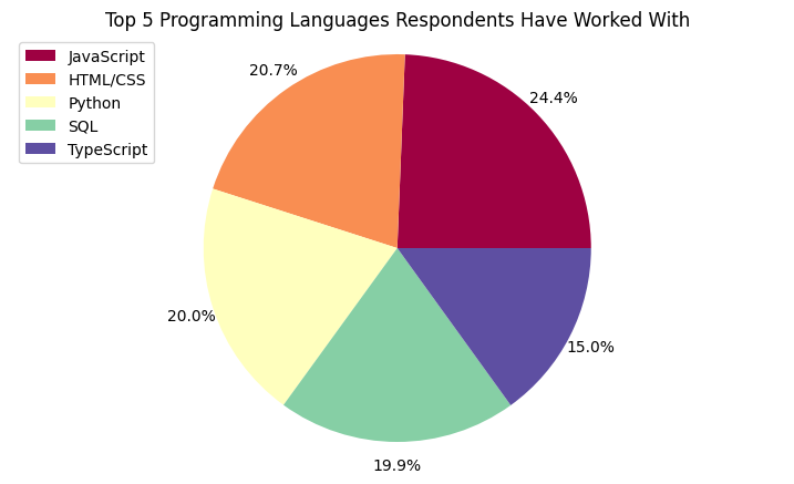
2.1 Pie Chart for Top 5 Programming Languages Respondents Have Worked With
The LanguageHaveWorkedWith column contains the programming languages that respondents have experience with. We’ll plot a pie chart to display the composition of the top 5 languages.
##Write your code here
dummies = df['LanguageHaveWorkedWith'].str.get_dummies(sep=';')
# Count total occurrences and sort
counts = dummies.sum().sort_values(ascending=False)
top5lang = counts.iloc[:5]

top5lang.plot(kind='pie',
              figsize=(9, 5),
              autopct='%1.1f%%', # add in percentages
              labels=None,
              startangle=0,
              pctdistance=1.12,  # the ratio between the center of each pie slice and the start of the text
              shadow=False,
              colormap='Spectral')

plt.title('Top 5 Programming Languages Respondents Have Worked With')
plt.axis('equal') # Sets the pie chart to look like a circle
plt.legend(labels=top5lang.index, loc='upper left')

plt.show()
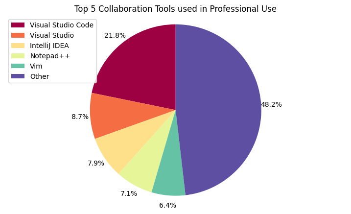
2.2 Pie Chart for Top Collaboration Tools used in Professional Use
Using the NEWCollabToolsHaveWorkedWith column, we’ll identify and visualize the top collaboration tools respondents use in their professional work.
##Write your code here
dummies = df['NEWCollabToolsHaveWorkedWith'].str.get_dummies(sep=';')
# Count total occurrences and sort
counts = dummies.sum().sort_values(ascending=False)
# Build Top 5 + Other
top5 = counts.iloc[:5]
other = counts.iloc[5:].sum()
coltoolsp = pd.concat([top5, pd.Series({'Other': other})])

coltoolsp.plot(kind='pie',
              figsize=(9, 5),
              autopct='%1.1f%%', # add in percentages
              labels=None,
              startangle=90,
              pctdistance=1.12,  # the ratio between the center of each pie slice and the start of the text
              shadow=False,
              colormap='Spectral')

plt.title('Top 5 Collaboration Tools used in Professional Use')
plt.axis('equal') # Sets the pie chart to look like a circle
wrapped_labels = ['\n'.join(textwrap.wrap(label, 20)) for label in coltoolsp.index]
plt.legend(labels=wrapped_labels, loc='upper left')

plt.show()
Task 3: Analyzing and Interpreting Composition
In this task, you will create additional pie charts to analyze specific aspects of the survey data. Use pandas and matplotlib to complete each task and interpret the findings.
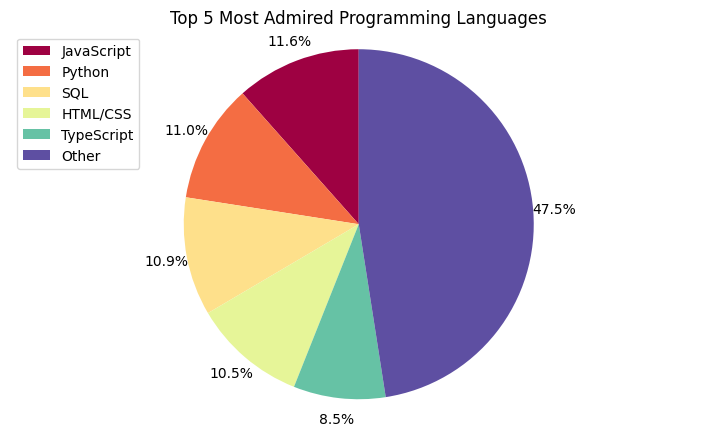
3.1 Pie Chart of Respondents Most Admired Programming Languages
The LanguageAdmired column lists the programming languages respondents admire most. Create a pie chart to visualize the top 5 admired languages.
##Write your code here
dummies = df['LanguageAdmired'].str.get_dummies(sep=';')
# Count total occurrences and sort
counts = dummies.sum().sort_values(ascending=False)
# Build Top 5 + Other
top5 = counts.iloc[:5]
other = counts.iloc[5:].sum()
langadmp = pd.concat([top5, pd.Series({'Other': other})])

langadmp.plot(kind='pie',
              figsize=(9, 5),
              autopct='%1.1f%%', # add in percentages
              labels=None,
              startangle=90,
              pctdistance=1.12,  # the ratio between the center of each pie slice and the start of the text
              shadow=False,
              colormap='Spectral')

plt.title('Top 5 Most Admired Programming Languages')
plt.axis('equal') # Sets the pie chart to look like a circle
plt.legend(labels=langadmp.index, loc='upper left')

plt.show()
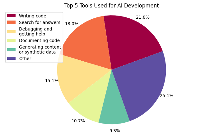
3.2 Pie Chart of Tools Used for AI Development
Using the AIToolCurrently Using column, create a pie chart to visualize the top 5 tools developers are currently using for AI development.
##Write your code here
dummies = df['AIToolCurrently Using'].str.get_dummies(sep=';')
# Count total occurrences and sort
counts = dummies.sum().sort_values(ascending=False)
# Build Top 5 + Other
top5 = counts.iloc[:5]
other = counts.iloc[5:].sum()
aitoolp = pd.concat([top5, pd.Series({'Other': other})])

aitoolp.plot(kind='pie',
              figsize=(9, 5),
              autopct='%1.1f%%', # add in percentages
              labels=None,
              startangle=20,
              pctdistance=1.12,  # the ratio between the center of each pie slice and the start of the text
              shadow=False,
              colormap='Spectral')

plt.title('Top 5 Tools Used for AI Development')
plt.axis('equal') # Sets the pie chart to look like a circle
wrapped_labels = ['\n'.join(textwrap.wrap(label, 20)) for label in aitoolp.index]
plt.legend(labels=wrapped_labels, loc='upper left')

plt.show()
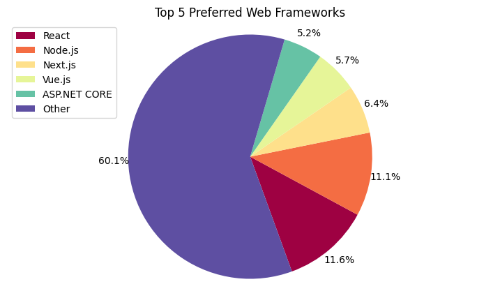
3.3 Pie Chart for Preferred Web Frameworks
The WebframeWantToWorkWith column includes web frameworks that respondents are interested in working with. Visualize the top 5 frameworks in a pie chart.
##Write your code here
dummies = df['WebframeWantToWorkWith'].str.get_dummies(sep=';')
# Count total occurrences and sort
counts = dummies.sum().sort_values(ascending=False)
# Build Top 5 + Other
top5 = counts.iloc[:5]
other = counts.iloc[5:].sum()
webfrtoworkp = pd.concat([top5, pd.Series({'Other': other})])

webfrtoworkp.plot(kind='pie',
              figsize=(9, 5),
              autopct='%1.1f%%', # add in percentages
              labels=None,
              startangle=-70,
              pctdistance=1.12,  # the ratio between the center of each pie slice and the start of the text
              shadow=False,
              colormap='Spectral')

plt.title('Top 5 Preferred Web Frameworks')
plt.axis('equal') # Sets the pie chart to look like a circle
wrapped_labels = ['\n'.join(textwrap.wrap(label, 20)) for label in webfrtoworkp.index]
plt.legend(labels=wrapped_labels, loc='upper left')

plt.show()
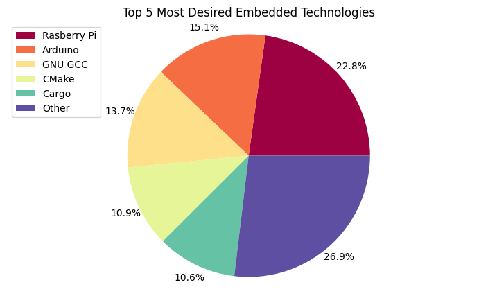
3.4 Pie Chart for Most Desired Embedded Technologies
Using the EmbeddedWantToWorkWith column, create a pie chart to show the top 5 most desired embedded technologies that respondents wish to work with.
##Write your code here
dummies = df['EmbeddedWantToWorkWith'].str.get_dummies(sep=';')
# Count total occurrences and sort
counts = dummies.sum().sort_values(ascending=False)
# Build Top 5 + Other
top5 = counts.iloc[:5]
other = counts.iloc[5:].sum()
embtoworkp = pd.concat([top5, pd.Series({'Other': other})])

embtoworkp.plot(kind='pie',
              figsize=(9, 5),
              autopct='%1.1f%%', # add in percentages
              labels=None,
              startangle=0,
              pctdistance=1.12,  # the ratio between the center of each pie slice and the start of the text
              shadow=False,
              colormap='Spectral')

plt.title('Top 5 Most Desired Embedded Technologies')
plt.axis('equal') # Sets the pie chart to look like a circle
wrapped_labels = ['\n'.join(textwrap.wrap(label, 20)) for label in embtoworkp.index]
plt.legend(labels=wrapped_labels, loc='upper left')

plt.show()
Summary
After completing this lab, you will be able to:
- Create pie charts to visualize developer preferences across databases, programming languages, AI tools, and cloud platforms.
- Identify trends in technology usage, role distribution, and tool adoption through pie charts.
- Analyze and compare data composition across various categories to gain insights into developer preferences.
Authors:
Ayushi Jain
Other Contributors:
- Rav Ahuja
- Lakshmi Holla
- Malika
Copyright © IBM Corporation. All rights reserved.