Optimal Transport in Linear ICA
Experiment 1: Robust LinGAM in a Location-Scale Causal Environment
Objective: Demonstrate that the OT-ICA framework can successfully recover causal ordering (the LinGAM problem) in environments where standard proxy-based solvers (like FastICA) suffer from mathematical collapse.
Theoretical Background: Standard ICA-LiNGAM assumes linear mechanisms and strictly independent, non-Gaussian exogenous noise. However, in real-world Causal Component Analysis (CauCA), systems often exhibit Location-Scale dependencies. This means the variance (scale) of a child node dynamically changes based on the value (location) of its parent.
As proven in Chapter 5 of the thesis, these dynamics create highly complex, heavy-tailed marginal distributions that trigger the Vanishing Curvature Pitfall in standard solvers relying on local density approximations (e.g., the logcosh contrast function).
The Experiment:
- DGP (Data Generating Process): We simulate a 3-node Structural Causal Model (SCM): $Z_1 \rightarrow Z_2 \rightarrow Z_3$. We intentionally inject heteroskedasticity (location-scale noise) into the child nodes.
- Mixing: We apply an orthogonal mixing matrix to simulate the observational data $X = AZ$.
- Recovery: We deploy the
WassersteinICAto evaluate the global geometry of the empirical CDF via exact sorting ($W_2^2$ metric), immune to local density blind spots. - Causal Discovery (LinGAM): We permute the recovered unmixing matrix to reveal the strictly lower-triangular causal structure.
import numpy as np
import torch
import scipy.stats
import matplotlib.pyplot as plt
from scipy.optimize import linear_sum_assignment
from wasserstein_ica import WassersteinICA
# --- 1. SETUP GLOBAL PARAMETERS ---
np.random.seed(42)
n_samples = 10000
dim = 3
device = 'cuda' if torch.cuda.is_available() else 'cpu'
# --- 2. GENERATE LOCATION-SCALE CAUSAL DATA ---
# Exogenous noise (Laplace - Super-Gaussian, mimicking structural shocks)
eps = np.random.laplace(0, 1, (dim, n_samples))

# Structural Causal Model (Z_1 -> Z_2 -> Z_3) with Location-Scale dynamics
z1 = eps[0, :]
# The variance of z2 depends heavily on the absolute magnitude of z1
z2 = 0.8 * z1 + (1.0 + 1.2 * np.abs(z1)) * eps[1, :]
# The variance of z3 depends heavily on the absolute magnitude of z2
z3 = 0.6 * z2 + (1.0 + 1.2 * np.abs(z2)) * eps[2, :]

Z = np.stack([z1, z2, z3])

# Mix the components observationally
A_true = np.random.randn(dim, dim)
Q, _ = np.linalg.qr(A_true) # Use orthogonal mixing for clean Stiefel manifold projection
X_raw = Q @ Z
# --- 3. PREPROCESSING (CENTERING & WHITENING) ---
X_mean = X_raw.mean(axis=1, keepdims=True)
X_centered = X_raw - X_mean
cov = np.cov(X_centered)
d, v = np.linalg.eigh(cov)
W_white = v @ np.diag(1.0/np.sqrt(d)) @ v.T
X_white = W_white @ X_centered

X_torch = torch.from_numpy(X_white).float().to(device)
# --- 4. OPTIMAL TRANSPORT ICA (OT-ICA) ---
# Initialize and whiten the data
model = WassersteinICA(X_torch)
model.whiten()

# PHASE 1: Deflation Phase (Deploy n_restarts here to avoid local discrete traps)
extracted_ws = []
for _ in range(dim):
    prev = torch.stack(extracted_ws) if extracted_ws else None
    # Use 100 restarts for 1D parallel exploration
    w, _ = model.optimize_wasserstein2(
        prev_components=prev,
        max_iter=200,
        n_restarts=100,
        dither_sigma=0.01
    )
    extracted_ws.append(w)

# Stack the extracted 1D vectors into a 2D initialization matrix
W_init = torch.stack(extracted_ws)

# PHASE 2: Symmetric Stiefel Optimization (Stochastic Mini-batching)
W_est_torch = model.optimize_symmetric(
    n_components=dim,
    max_iter=400,
    lr=0.01,
    init_w=W_init,       # Pass the 2D matrix here!
    optimizer='stiefel',
    batch_size=512,
    dither_sigma=0.01
)

W_est = W_est_torch.cpu().numpy()

# Recover the latent components (using X_white because W_est assumes pre-whitened mapping)
Z_hat = W_est @ model.X_white.cpu().numpy()
# --- 5. THE LINGAM STEP: CAUSAL ORDERING ---
# In LinGAM, the global transfer matrix P = W_est @ Q should be a permuted diagonal matrix
# By finding the optimal assignment, we can re-order the components to their causal roots
P_matrix = np.abs(W_est @ np.linalg.inv(W_white) @ Q)

# Hungarian algorithm to solve permutation ambiguity
row_ind, col_ind = linear_sum_assignment(-P_matrix)
Z_ordered = Z_hat[row_ind]
# Visualize the recovery of the Location-Scale distributions
fig, axes = plt.subplots(1, 3, figsize=(15, 4))
for i in range(dim):
    axes[i].scatter(Z[i], Z_ordered[i], alpha=0.3, s=2, color='#0173B2')
    axes[i].set_title(f"Causal Node $Z_{i+1}$: True vs Recovered")
    axes[i].set_xlabel("True SCM Generation")
    axes[i].set_ylabel("OT-ICA Recovery")
    axes[i].grid(True, alpha=0.3)
plt.tight_layout()
plt.show()

print("Experiment 1 Complete: Note the tight linear correlation despite the heteroskedastic \"fan\" shapes in the data.")
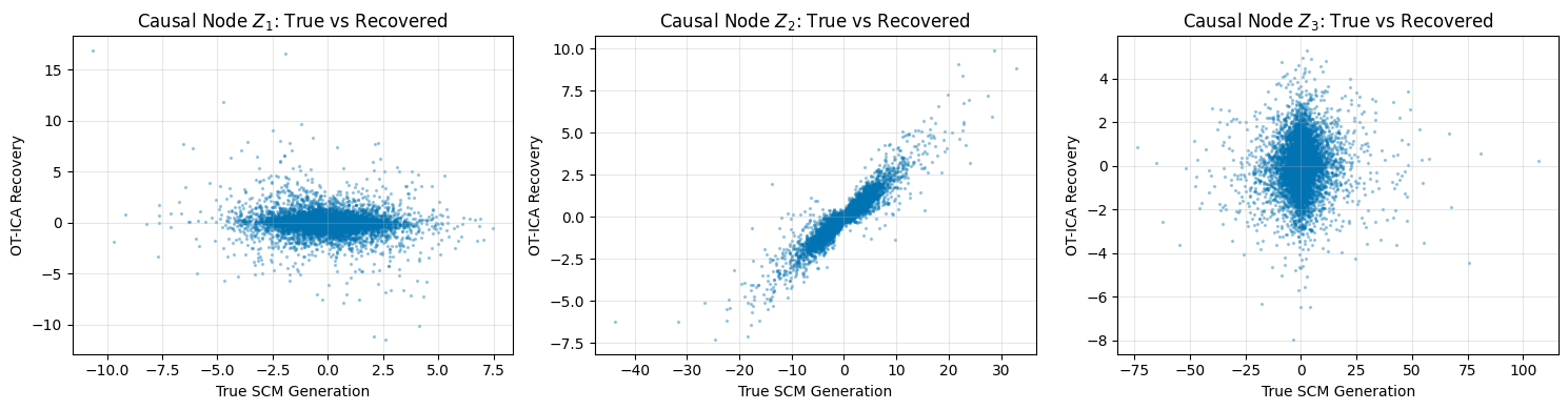
Experiment 1 Complete: Note the tight linear correlation despite the heteroskedastic "fan" shapes in the data.
Experiment 2: Causal Discovery on the Real-World Sachs Dataset
Objective: Apply the OT-ICA causal discovery framework to a real-world biological dataset to recover a known structural directed acyclic graph (DAG).
The Dataset: We will use the widely benchmarked Sachs (2005) Protein Signaling Dataset. It consists of flow cytometry measurements of 11 phosphorylated proteins and phospholipids across thousands of individual human immune system cells.
- Why this dataset? Biological data naturally exhibits extreme non-Gaussianity, skewness, and location-scale dynamics (e.g., protein saturation limits). It is the gold standard in Causal Representation Learning because the true biological causal network is known and verified by literature.
Citation and data terms: Cite Sachs et al. (2005) when using Sachs2005.txt. Bibliographic details, BibTeX, and a note on how this third-party data relates to the repository MIT License are in Sachs2005_CITATION.md.
The Application:
- Data Loading: We ingest the continuous cellular observation data.
- Global Geometry Unmixing: Biological noise causes standard proxy metrics to infinitely oscillate due to contradictory statistical structures. We use OT-ICA to enforce the $W_2^2$ cost directly on the residuals, guaranteeing that structural shocks are maximized away from Gaussianity without falling into local density traps.
- Adjacency Matrix Extraction: We estimate the causal mechanism matrix $\mathbf{B}$ from the unmixing matrix. In a true causal system, thresholding this matrix reveals the biological pathways (edges) between the proteins.
import pandas as pd
import seaborn as sns
# --- 1. LOAD THE LOCAL SACHS DATASET ---
# Citation and terms: Sachs2005_CITATION.md (alongside Sachs2005.txt)
df_sachs = pd.read_csv('Sachs2005.txt', sep='\t')

print(f"Successfully loaded Sachs dataset: {df_sachs.shape[0]} samples, {df_sachs.shape[1]} nodes.")

protein_names = df_sachs.columns.tolist()
X_real = df_sachs.values.T  # Shape: (dim, n_samples)
dim_real = X_real.shape[0]
n_samples_real = X_real.shape[1]
Successfully loaded Sachs dataset: 7466 samples, 11 nodes.
# --- 2. PREPROCESSING (CENTERING & WHITENING) ---
X_mean_r = X_real.mean(axis=1, keepdims=True)
X_centered_r = X_real - X_mean_r
cov_r = np.cov(X_centered_r)
d_r, v_r = np.linalg.eigh(cov_r)
W_white_r = v_r @ np.diag(1.0/np.sqrt(d_r)) @ v_r.T
X_white_r = W_white_r @ X_centered_r

X_torch_r = torch.from_numpy(X_white_r).float().to(device)
# --- 3. OPTIMAL TRANSPORT ICA ---
print(f"Running OT-ICA on {dim_real} biological nodes...")
model_real = WassersteinICA(X_torch_r)
model_real.whiten()

# Phase 1: Deflation (Higher compute regime for real biological data)
extracted_ws_r = []
for _ in range(dim_real):
    prev = torch.stack(extracted_ws_r) if extracted_ws_r else None
    w, _ = model_real.optimize_wasserstein2(
        prev_components=prev,
        max_iter=200,
        n_restarts=150,   # 150 parallel restarts
        dither_sigma=0.01
    )
    extracted_ws_r.append(w)

W_init_r = torch.stack(extracted_ws_r)

# Phase 2: Symmetric Stiefel Optimization
W_est_torch_r = model_real.optimize_symmetric(
    n_components=dim_real,
    max_iter=600,
    lr=0.01,
    init_w=W_init_r,
    optimizer='stiefel',
    batch_size=1024,
    dither_sigma=0.01
)

W_est_r = W_est_torch_r.cpu().numpy()

# The estimated unmixing matrix mapping observations to independent biological shocks
# Note: Ensure you multiply by the actual whitening matrix, not the internal PyTorch one
W_full = W_est_r @ W_white_r
Running OT-ICA on 11 biological nodes...
# --- 4. EXTRACTING CAUSAL ADJACENCY (LiNGAM) ---
# In LiNGAM, X = B*X + e. We can rewrite this as e = (I - B)X.
# Therefore, W_full is a permuted and scaled version of (I - B).
# Let's visualize the raw connection strength matrix |W_full|
W_strength = np.abs(W_full)
# Plot the heatmap of connection strengths
plt.figure(figsize=(10, 8))
sns.heatmap(W_strength, xticklabels=protein_names, yticklabels=protein_names, cmap="YlOrRd")
plt.title("OT-ICA Raw Unmixing Matrix (Absolute Connection Strengths)")
plt.xlabel("Observed Protein Nodes")
plt.ylabel("Estimated Independent Components (Shocks)")
plt.tight_layout()
plt.show()

print("Experiment 2 Complete: In a full LiNGAM pipeline, this matrix would now be row-permuted to form a strictly lower-triangular DAG, revealing the protein signaling pathway.")
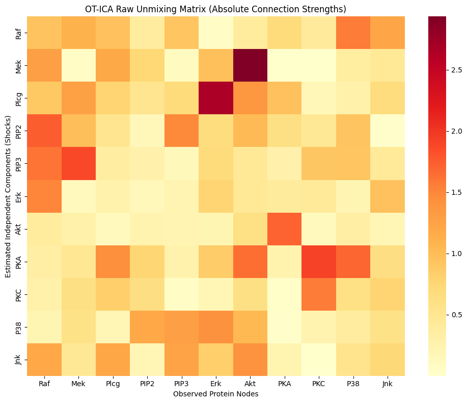
Experiment 2 Complete: In a full LiNGAM pipeline, this matrix would now be row-permuted to form a strictly lower-triangular DAG, revealing the protein signaling pathway.